This document defines a specification for both a core system
dynamics (SD) language and its representation in XML and thus provides a common
structure for describing SD models.
In the Spring 2003 System Dynamics Society newsletter, Jim
Hines proposed that there be a common interchange format for system dynamics
models. Magne Myrtveit originally proposed such an idea at the 1995 International
System Dynamics Conference (ISDC), but Jim hoped to revive interest in the idea
and chose the name SMILE (Simulation Model Interchange LanguagE) to keep people
lighthearted. The benefits Jim proposed at the time were:
- Sharing of models can lead to greater increases of
knowledge and sharing of ideas.
- On-line repositories could be built to facilitate learning.
- Open standards lead to better acceptance in larger
corporations as it minimizes their risk with specific vendors.
- It spurs innovation by allowing non-vendors to develop
add-ons.
To this formidable list, the following can be added:
- It allows the creation of a historical record of important
works that everyone has access to.
- It allows vendors to expand their market base because
suddenly their unique features (and let’s be honest – each of the three
major players has unique competencies) are available to all system
dynamics modelers.
Vedat Diker and Robert Allen later presented a poster at the
2005 ISDC that proposed a working group be formed and that XML be the working
language for the standard, leading to the name XMILE (XML Modeling Interchange
LanguagE). During the first meeting of the Information Systems Special
Interest Group (SIG) at the 2006 ISDC, Karim Chichakly volunteered to develop
the draft XMILE specification, which he presented at the 2007 ISDC. Several
drafts later, the OASIS XMILE Technical Committee (TC) was formed in June 2013
to standardize the specification across all industries. This document is the
result of that TC’s work.
This specification defines the XMILE specification version
1.0.
The key words “MUST”, “MUST NOT”, “REQUIRED”, “SHALL”, “SHALL
NOT”, “SHOULD”, “SHOULD NOT”, “RECOMMENDED”, “MAY”, and “OPTIONAL” in this
document are to be interpreted as described in [RFC2119].
[RFC2119] Bradner,
S., “Key words for use in RFCs to Indicate Requirement Levels”, BCP 14, RFC
2119, March 1997. http://www.ietf.org/rfc/rfc2119.txt.
[Reference] [Full reference citation]
[Reference] [Full reference citation]
NOTE: The proper format for citation of technical
work produced by an OASIS TC (whether Standards Track or Non-Standards Track)
is:
[Citation Label]
Work Product title
(italicized). Approval date (DD Month YYYY). OASIS Stage
Identifier and Revision Number (e.g.,
OASIS Committee Specification Draft 01). Principal URI (version-specific URI, e.g., with filename
component: somespec-v1.0-csd01.html).
For example:
[OpenDoc-1.2] Open Document Format for Office Applications
(OpenDocument) Version 1.2. 19 January 2011. OASIS Committee Specification
Draft 07. http://docs.oasis-open.org/office/v1.2/csd07/OpenDocument-v1.2-csd07.html.
[CAP-1.2] Common
Alerting Protocol Version 1.2. 01 July 2010. OASIS Standard. http://docs.oasis-open.org/emergency/cap/v1.2/CAP-v1.2-os.html.
A XMILE document is a container for information about a
modeling project, with a well-specified structure. The document must be encoded
in UTF-8. The entire XMILE document is enclosed within a <xmile> tag as
follows:
<xmile version="1.0"
xmlns="http://docs.oasis-open.org/xmile/ns/XMILE/v1.0">
...
</xmile>
The version number MUST refer to the version of XMILE used
(presently 1.0). The XML namespace refers to tags and attributes used in this
specification. Both of these attributes are required. Inside of the
<xmile> tag are a number of top-level tags, listed below. These tags are
marked req (a single instance is REQUIRED), opt (a single instance is
OPTIONAL), * (zero or more tags MAY occur) and + (one or more tags MAY occur).
Top level tags MAY occur in any order, but are RECOMMENDED to occur in the
following order:
·
<header>
(req) - information about the origin of the model and required capabilities.
·
<sim_specs>
(opt) - default simulation specifications for this model.
·
<model_units>
(opt) - definitions of units used in this model.
·
<dimensions>
(opt) - definitions of array dimensions specific to this model.
·
<behavior>
(opt) - simulation style definitions that are inherited/cascaded through all
models defined in this XMILE document
·
<style>
(opt) - display style definitions that are inherited/cascaded through all
models defined in this XMILE document.
·
<data>
(opt) - definitions of persistent data import/export connections..
·
<model>+
- definition of model equations and (optionally) diagrams.
·
<macro>*
- definition of macros that can be used in model equations.
These tags/document sections are specified in the subsequent
sections of this chapter, after XMILE namespaces are discussed.
When an XMILE file includes references to models contained
in separate files or at a specific URL, each such file may contain overlapping
information, most commonly in sim_specs, model_units and dimensions. When such
overlap is consistent, combining parts is done by taking the union of the
different component files. When an inconsistency is found, (for example, a
dimension with two distinct definitions) software reading the files MUST
resolve the inconsistency and SHOULD provide user feedback in doing so. Some
inconsistencies, such as conflicting Macro or Model names MUST be resolved as
detailed in section 1.11.3.
There are four categories of namespaces in play in a XMILE
document - XML tag namespaces, Variable namespace, Function namespace and Unit
namespaces. XML tag namespaces and Unit namespaces are independent, but
Variable and Function namespaces interact.
XML tag namespaces are global. Unadorned tags are described
in detail in the various sections of this document and provision for vendor
specific additions are also detailed.
Each XMILE project has a single Unit namespace against which
all Unit Definitions and Equation Units are resolved. The Unit namespace is
separate from any other namespaces and this means that the variables of units
and variable or function names can overlap (for example someone might use
Ounce/Min and define Min as an alias of Minute even though MIN is a reserved
function name). Because this namespace crosses models Unit Definitions
contained in separate files must be combined into this namespace.
The Function namespace combines global definitions (all
functions defined here along with vendor specified functions) with project
specific definitions through Macros. In every case, however, the names MUST be
uniquely resolvable within a project independent of the model in which they
appear. It is not possible, for example, to give the same macro name two
different definitions in separate models. Dimension names, though conceptually
part of the Variable namespace, behave the same way and MUST be unique across a
project.
Variable names are resolved within models, but in the same
context as functions and therefore can't overlap. It is not, for example,
possible to have a variable named MIN as this is a reserved function name.
Similarly, if the macro BIGGEST has been defined, no variable may be given the
name BIGGEST. It is, however, possible, to have the same variable name appear
in different models. For example if you have a project with one model
MyCompany and another model Competitors, both could contain the variable profit
(with MyCompany.profit and Competitors.profit the way to refer to that variable
from different models).
One final subtlety in namespaces is that Dimension names, in
turn, define their own Element namespace. Thus, even through Array Dimension
names must be unique, they can have overlapping Element names and the Element
names can be the same as Variable names. Element names are resolved by context
when they appear inside square brackets of a variable and can be used in
context by prefixing them with the array dimension name (as in Location.Boston,
where Location is a Dimension name with element Boston).
The XML tag for the file header is <header>. The REQUIRED sub-tags
are:
·
XMILE options: <options>
(defined below)
·
Vendor name: <vendor>
w/company name
·
Product name: <product
version="…" lang="…"> w/product name – the
product version number is required. The language code is optional (default:
English) and describes the language used for variable names and comments.
Language codes are described by ISO 639-1 unless the language is not there, in
which case the ISO 639-2 code should be used (e.g., for Hawaiian).
OPTIONAL sub-tags include:
·
Model name: <name>
w/name
·
Model version: <version>
w/version information
·
Model caption: <caption>
w/caption
·
Picture of the model in JPG, GIF, TIF, or PNG format: <image resource=””>.
The resource
attribute is optional and may specify a relative file path, an absolute file
path, or an URL. The picture data may
also be embedded inside the <image> tag in Data URI format, using base64 encoding.
·
Author name: <author>
w/author name
·
Company name: <affiliation>
w/company name
·
Client name: <client>
w/client name
·
Copyright notice: <copyright> w/copyright information
·
Contact information (e-mail, phone, mailing address, web site):
<contact>
block w/contact information broken into <address>,
<phone>,
<fax>, <email>, and <website>,
all optional
·
Date created: <created>
whose contents MUST be in ISO 8601 format, e.g. “ 2014-08-10”.
·
Date modified: <modified>
whose contents MUST be in ISO 8601 format, as well
·
Model universally unique ID: <uuid> where the ID MUST be in
IETF RFC4122 format (84-4-4-12 hex digits with the dashes)
·
Includes: <includes>
section with a list of included files or URLs. This is specified in more detail
in Section 2.11.
The XMILE options appear under the tag <options>. This is a list of
functionality that is used in models in the current document that may not be
included in all implementations. If the current document makes use of any of
the following functionality, it SHOULD be be listed under the <options>
tag. The available options are:
<uses_conveyor/>
<uses_queue/>
<uses_arrays/>
<uses_submodels/>
<uses_macros/>
<uses_event_posters/>
<has_model_view/>
<uses_outputs/>
<uses_inputs/>
<uses_annotation/>
There is one OPTIONAL attribute for the <options>
tag:
·
Namespace: namespace="…"
with XMILE namespaces, separated by commas. For example, namespace="std, isee" means
try to resolve unrecognized identifiers against the std namespace first, and then against
the isee
namespace. (default: std)
The <uses_arrays>
tag has one REQUIRED attribute and OPTIONAL attribute:
·
Required: Specify the maximum dimensions used by any variable in
the model: maximum_dimensions.
·
Optional: Specify the value returned when an index is invalid: invalid_index_value="…"
with NaN/0 (default: 0)
The <uses_macros>
tag has several REQUIRED attributes:
·
Has macros which are recursive (directly or indirectly): recursive_macros="…"
with true/false.
·
Defines option filters: option_filters="…" with
true/false.
The <uses_conveyor>
tag has two OPTIONAL attributes:
·
Has conveyors that arrest: arrest="…" with true/false
(default: false)
·
Has conveyor leakages: leak="…" with true/false
(default: false)
The <uses_queue>
tag has one OPTIONAL attribute:
·
Has queue overflows: overflow="…" with true/false
(default: false)
The <uses_event_posters>
tag has one OPTIONAL attribute:
·
Has messages: messages="…"
with true/false (default: false)
The <has_model_view>
tag notes whether the XMILE file contains 1 or more <view> sections containing a visual
representation of the model. Note that all models, even those without
diagrams, SHOULD be simulateable by any software which supports XMILE.
The <uses_outputs>
tag implies both time-series graphs and tables are included. It has three
OPTIONAL attributes:
·
Has numeric display: numeric_display="…" with
true/false (default: false)
·
Has lamp: lamp="…"
with true/false (default: false)
·
Has gauge: gauge="…"
with true/false (default: false)
The <uses_inputs>
tag implies sliders, knobs, switches, and option groups are included. It has three
OPTIONAL attributes:
·
Has numeric input: numeric_input="…" with true/false (default:
false)
·
Has list input: list="…" with true/false (default: false)
·
Has graphical input: graphical_input="…" with
true/false (default: false)
The <uses_annotation>
tag implies text boxes, graphics frames, and buttons are included.
A sample options block appears below:
<options namespace="std, isee">
<uses_conveyors leak="true"/> <!-- has conveyors, some
leak -->
<uses_arrays
maximum_dimensions=”2”/> <!-- has 2D arrays -->
<has_model_view/> <!--
has diagram of model -->
</options>
Every XMILE file MUST contain at least one set of simulation
specifications, either as a top-level tag under <xmile> or as a child of the root model.
Note that simulation specifications can recur in each Model section to override
specific global defaults. Great care should be taken in these situations to
avoid nonsensical results.
The simulation specifications block is defined with the tag <sim_specs>.
The following properties are REQUIRED:
·
Start time: <start>
w/time
·
Stop time: <stop>
w/time (after start time)
There are several additional OPTIONAL attributes and
properties with appropriate defaults:
·
Step size: <dt>
w/value (default: 1)
Optionally specified as the integer reciprocal of DT (for DT <= 1 only) with
an attribute of <dt>:
reciprocal="…"
with true/false (default: false)
·
Integration method: method="…" w/XMILE name (default: euler)
·
Unit of time: time_units="…"
w/Name (empty default)
·
Pause interval: pause="…" w/interval (default: infinity – can
be ignored)
·
Run selected groups or modules: <run by="…"> with run
type either: all,
group, or module (default:
all, i.e., run entire model). Which groups or modules to run are identified by
run
attributes on the group or model.
All user-specified model unit
definitions are specified in the <model_units> tag as shown below:
<model_units>
<unit
name="models_per_person_per_year">
<eqn>models/person/year</eqn> <!--
name, equation -->
</unit>
<unit
name="Rabbits">
<alias>Rabbit</alias> <!--
name, alias -->
</unit>
<unit
name="models_per_year">
<eqn>models/year</eqn> <!--
name, eqn, alias -->
<alias>model_per_year</alias>
<alias>mpy</alias>
</unit>
<unit name="Joules"
disabled="true"> <!-- disabled unit -->
<alias>J</alias>
</unit>
</model_units>
All unit definitions MUST contain a name, possibly an
equation, and 0 or more aliases (Including a unit definition with only a name
is valid but discouraged). Unit equations (<eqn> tag) are defined with XMILE
unit expressions. One <alias>
tag with the name of the alias appears for each distinct unit alias. A unit
with the attribute disabled set to true MUST NOT be included in the unit
substitution process. It is included to override a Unit Definition that may be
built into the software or specified as a preference by the user.
Vendor-provided unit definitions not used in a model are NOT
REQUIRED to appear in the model, but SHOULD be made available in this same
format in a vendor-specific library.
When the <uses_arrays>
XMILE option is set, a list of dimension names is REQUIRED. These dimension
names must be consistent across all models. The set of dimension names appear
within a <dimensions>
block as shown in the example below.
<dimensions>
<dim name="N"
size="5"/> <!-- numbered indices -->
<dim
name="Location"> <!-- named indices -->
<elem
name="Boston"/> <!-- name of 1st index -->
<elem
name="Chicago"/> <!-- name of 2nd index -->
<elem name="LA"/> <!--
name of 3rd index -->
</dim>
</dimensions>
Each dimension name is identified with a <dim> tag and
a REQUIRED name. If the elements are not named, a size attribute greater or
equal to one MUST be given. If the elements have names, they appear in order in
<elem>
nodes. The dimension size MUST NOT appear when elements have names as the
number of element names always determines the size of such dimensions.
Every XMILE file MAY include behavior information to set
default options that affect the simulation of model entities. This is usually
used in combination with macros to change some aspect of a given type of
entity’s performance, for example, setting all stocks to be non-negative.
The behavior information
cascades across four levels from the entity outwards, with the actual entity
behavior defined by the first occurrence of a behavior definition for that
behavior property:
1. Behaviors
for the given entity
2. Behaviors
for the entire model (affects only that Model section)
3. Behaviors
for the entire model file (affects all Model sections)
4. Default
XMILE-defined behaviors when a default appears in this specification
The behavior block begins with the <behavior> tag. Within this block,
any known object can have its attributes set globally (but overridden locally)
using its own modifier tags. Global settings that apply to everything are
specified directly on the <behavior>
tag or in nodes below it. This is true for <behavior> tags that appear within
the <model>
tag as well. For example, all entities (particularly stocks and flows) can be
set to be non-negative by default:
<behavior>
<non_negative/>
</behavior>
Only stocks or only flows can
also be set to non-negative by default (flows in this example):
<behavior>
<flow>
<non_negative/>
</flow>
</behavior>
Every XMILE file MAY include style information to set
default options for display objects. Being style information, this mostly
belongs to the Presentation section (5.3), which describes the display and
layout of XMILE files.
The style information is cascading across four levels from
the entity outwards, with the actual entity style defined by the first
occurrence of a style definition for that style property:
1. Styles for
the given entity
2. Styles for
a specific view
3. Styles for
a collection of views
4. Default
XMILE-defined styles when a default appears in this specification
The style information usually includes program defaults when
they differ from the standard, though it can also be used for file-specific
file-wide settings. Whenever possible, style information uses standard CSS
syntax and keywords recast into XML attributes and nodes.
The style block begins with the <style> tag. Within this block,
any known object can have its attributes set globally (but overridden locally)
using its own modifier tags. Global settings that apply to everything are
specified directly on the <style>
tag or in nodes below it; this is true for <style> tags that appear within
the <views> tag
as well. For example, the following sets the color of objects within all models
to blue and the background to white:
<style color="blue"
background="white"/>
Unless otherwise indicated or specified, style information
appears in XML attributes. For example, font_family would be an attribute.
These changes can also be
applied directly to objects (again as a child to a <style> tag), e.g.,
<style
color="blue" background="white">
<connector
color="magenta">
</style>
Note that when style information applies to a specific
object, that style cannot be overridden at a lower level (e.g., within a view)
by a change to the overall style (i.e., by the options on the <style> tag).
Using the example above, to override the color of connectors at a lower level
(e.g., the Display), the <connector>
tag must explicitly appear in that level’s style block. If it does not appear
there, connectors will be magenta at that level by default, even if the style
block at that level sets the default color of all objects to green. In other
words, object-specific styles at any level above an object take precedence over
an overall style defined at any lower level.
Persistent data import/export connections are defined within
the OPTIONAL <data>
tag, which contains one <import>
tag for each data import connection and one <export> tag for each data export
connection. Both tags include the following properties (the first four are
optional):
·
Type: type="…"
with “CSV”, “Excel”, or “XML” (default: CSV)
·
Enabled state: enabled="…"
with true/false (default: true)
·
How often: frequency="…"
with either “on_demand” or “automatic” (default: automatic, i.e., whenever the
data changes)
·
Data orientation: orientation="…" with either “horizontal” or
“vertical” (default: vertical)
·
Source (import) or destination (export) location: resource="…".
A resource can be a relative file path, an absolute file path, or an URL.
·
For Excel only, worksheet name: worksheet="…" with worksheet
name
The <export>
also specifies both the optional export interval and one of two sources of the
data:
·
Export interval: interval="…" specifying how
often, in model time, to export values during the simulation; use "DT" to
export every DT (default: 0, meaning only once)
·
<all/>
to export all model variables or <table uid="…"/> to just export the
variables named in the table (note that any array element in the table will
export the entire array when interval is set to zero). The <table> tag
has an optional attribute use_settings="…"
with a true/false value (default: false), which when true causes the table
settings for orientation, interval, and number formatting to be used (thus,
when it is set, neither orientation nor interval are meaningful, so should not
appear). The uid used for the table must be qualified by the name of the module
in which the table appears. If in the root a ‘.’ is prefixed to the name, same
as module qualified variable names.
Model tags define models that can either be simulated
directly, or instantiated inside of other models as a module. Chapter 4
contains the specification for <model> tags.
Macro tags define macros that can be used in model entity
equations. Chapter 4 contains the specification for <macro> tags.
XMILE files MAY link to other
XMILE files. This serves the following use cases:
(1) A
model can be split across multiple files, allowing submodels and other
components to be individually edited or versioned
(2) A
modeler may create a common library of submodels or macros and use them for
multiple models
(3) A
modeler may create a common style for models and include a common file for such
style in different projects
(4)
A
vendor may create a common library of macros with specific functionality used
by all models produced by that vendor's software.
Included files are specified with an <includes> tag which goes inside
of <header>
<header>
...
<includes>
<include
resource="http://systemdynamics.org/xmile/macros/standard-1.0.xml"
/>
<include
resource="http://systemdynamics.org/xmile/macros/extra-1.0.xml" />
</includes>
</header>
The included resource can be specified in multiple ways. Specifically,
the resource attribute can be specified with:
(1) URLs. By convention,
a file retrieved from a URL is assumed to be an unchanging resource and may be
cached. The file may also be provided automatically by the simulation software.
Example:
<include
resource="http://systemdynamics.org/xmile/macros/standard-1.0.xml"
/>
(2) Relative file paths.
Search relative to the location of the model file. This allows modelers to
distribute their models as a folder of related files. This is a
machine-independent path specification using "/" to separate
directories. The "*" indicates a wildcard. Files are not cached.
<include
resource="my-macro-library.xml" />
<include
resource="macros/my-macro-library.xml" />
<include
resource="macros/*" />
<include resource="macros/supplychain-*.xml"
/>
(3) Absolute file paths.
Similar to relative file paths except that the resource starts with
"/" or "file://". In such cases, the file path is loaded
from an absolute location on the local machine. Application programs may choose
to limit file access or base the root directory in a particular location (e.g.
a home directory) for security reasons. A platform-specific volume name (e.g.
"D:") may not be specified.
<include
resource="/library/my-macro-library.xml" />
<include
resource="file://library/my-macro-library.xml" />
If an
absolute file path does not resolve to a file, as a fallback, the final
filename in the path should be stripped off and that name used for a search
relative to the model file itself.
By convention, files included from URLs are assumed to be
standard libraries provided by a vendor, organization or modeler, and MUST
never change once public. Such files should be versioned in the form
LIBRARY-MAJOR.MINOR.xml, e.g. "standard-1.0.xml". Changes to the content
of such libraries will require the major or minor version number to be
incremented. The full URL, e.g.
“http://systemdynamics.org/xmile/macros/standard-1.0.xml” represents a unique
identifier for the content of this file. Consequently, software packages MAY cache
such libraries or come pre-bundled with libraries for particular vendors or
organizations. Downloading the libraries each time the model loads is
discouraged.
As a contrast, files specified with a file path
(particularly a relative file path) are assumed to be part of the model
distribution and SHOULD be reloaded each time the model is loaded. Version
numbers in the file name are allowed but not required.
The format of the included files is a simplified version of
the format of the primary model. The <header> tag is OPTIONAL, and if
included can omit required header attributes. The <options> tag is optional.
<xmile
version="1.0"
xmlns=" http://docs.oasis-open.org/xmile/ns/XMILE/v1.0">
<header>
</header>
<macro
name="LOG">
...
</macro>
<macro name="LOG10">
...
</macro>
</xmile>
<xmile version="1.0" level="2" xmlns="http://www.systemdynamics.org/XMILE">
<style>
...
</style>
</xmile>
<xmile version="1.0" level="2" xmlns="http://www.systemdynamics.org/XMILE">
<model>
...
</model>
</xmile>
Software packages MUST process included files before
simulation is started, and the content of included files MUST be merged into
the model environment before simulation. Specifically:
·
The <options>
tag options will be merged with the <options> from the primary model.
This means that if an included file specifies an option such as <uses_conveyor/>,
then the simulation SHOULD assume the entire model has the <uses_conveyor/>
option specified. When merging XMILE <options> the most specific of
each option will take priority.
·
Any <behavior>
and <style>
options specified at the top level of the included file will be merged into the
default styles from the primary model. This allows behaviors and styles to be
included from other files. When merging <behavior> and <style>
options, any behaviors and styles specified in the primary model will take
priority. (This allows the primary model to overwrite styles specified in the
included file).
·
<model>
and <macro> tags in the included file will be merged into the primary
model at the start of the model, in the order in which they appear in the list
of included files. If there are name conflicts between <model> and <macro> tags in the included file
and the primary model, the primary model will take priority. (This allows the
primary model to overwrite submodels or macros specified in the included file).
At their heart, system dynamics models are systems of
integral (or differential) equations. We start from that perspective in
defining the basic structure of the simulation language. Using this frame, a
model is composed of stocks, flows, and other equations necessary to compute
the flows or initialize the stocks which we will call inclusively auxiliaries.
Stocks are also often called levels or states, and flows are often called rates
or derivatives. All other computations can include constants, initialization
computations, data constructs, and other items that will be distinguished by
their defining equations - all will be referred to as auxiliaries. Stocks,
flows, and auxiliaries will be collectively referred to as variables.
We also base our computational definition on the assumption
that a model starts from some well-defined initial condition and then
computations progress forward in time. Other approaches, such as mixed initial
and terminal conditions or simulating backwards in time, can be applied to the
models specified in this document but will require extensions of the
specification to accommodate these differences.
We will refer to the computation used to determine the
values of variables over time as "the simulation." In later sections,
we will discuss solution techniques for integral equations, but for discussion
purposes we will use the notion that time is broken up into finite intervals
during this computation. We will call the time between these intervals DT,
corresponding the denominator in the notation often used in introductory
calculus courses. DT is directly analogous to Δt in the Riemann
sum. This discrete time terminology is often used for pedagogical purposes and
is also important in defining computation, especially with some of the added
constructs such as queues now common in many system dynamics models.
As a final note, all variables in XMILE models are floating
point numbers. It is recommended that software supporting XMILE use
double-precision floating point numbers as specified by IEEE 754. At a
minimum, such software should maintain at least single-precision floating point
numbers.
The following sections define the core system dynamics
language that is required to be XMILE-compliant.
Stocks accumulate. Their value at the start of the
simulation MUST be set as either a constant or with an initial equation. The
initial equation is evaluated only once, at the beginning of the simulation.
During the course of the simulation, the value of a stock is
increased by its inflows and decreased by its outflows. Using the discrete time
interval dt and subscripted text to represent a value at given time, we
can write
stockt = stockt
- dt + dt×(inflowst
- dt – outflowst - dt)
The above computation is notional, though it is used in one
of the specified integration techniques (Euler).
In specifying a stock, we list its inflows and outflows
separately as in:
stock: Population
inflows: births, immigration
outflows: deaths, emigration
eqn: 100
units: people
Flows represent rates of change of the stocks. They MUST be
defined using any algebraic expression as described in Section 3.3 or by using
a graphical function as described in Section 3.1.4.
During the course of a simulation, a flow’s value is
computed and used in the computation of levels as described. An example flow:
flow: births
eqn: Population*birth_rate
units: people/year
Auxiliaries allow the isolation of any algebraic function
that is used. They can both clarify a model and factor out important or
repeated calculations. They MUST be defined using any algebraic expression (including
a constant value), optionally in conjunction with a graphical function.
An example auxiliary:
aux: birth_rate
eqn: normal_birth_rate*food_availability_multiplier
units: people/person/year
Auxiliaries can also represent constants:
aux: normal_birth_rate
eqn: 0.04
units: people/person/year
Graphical functions are alternately called lookup functions
and table functions. They are used to describe an arbitrary relationship
between one input variable and one output variable. The domain of these
functions is consistently referred to as x and the range is consistently
referred to as y.
A graphical function MUST be defined either with an x-axis
scale and a set of y-values (evenly spaced across the given x-axis
scale) or with a set of x-y pairs. An example of a graphical
function using an x-axis scale with a set of y-values:
Graphical Function:
food_availability_multiplier_function
x scale: 0 to 1
y values: 0, 0.3, 0.55, 0.7, 0.83, 0.9, 0.95, 0.98, 0.99, 0.995,
1
As there are 11 y values, the x-axis also must
be divided into 11 values from zero to one, leading to an x-axis
interval of 0.1. The graph of this function appears below.
0 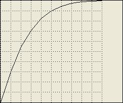
0 1
Distinct x-y pairs are intended for use when
the function cannot be properly represented by using a fixed interval along the
x-axis. Although not desired for the above graphical function, it can
be represented using a set of x-y pairs as follows:
Graphical Function:
food_availability_multiplier_function
x values: 0, 0.1, 0.2, 0.3, 0.4, 0.5, 0.6, 0.7, 0.8,
0.9, 1
y values: 0, 0.3, 0.55, 0.7, 0.83, 0.9, 0.95, 0.98, 0.99, 0.995,
1
The example graphical function above is continuous. There
are three types of graphical functions supported, with these names, which
define how intermediate and out-of-range values are calculated:
Name Description
continuous Intermediate
values are calculated with linear interpolation between the intermediate
points. Out-of-range values are the same as the closest endpoint (i.e, no
extrapolation is performed).
extrapolate Intermediate
values are calculated with linear interpolation between the intermediate
points. Out-of-range values are calculated with linear extrapolation from the
last two values at either end.
discrete Intermediate
values take on the value associated with the next lower x-coordinate
(also called a step-wise function). The last two points of a discrete graphical
function must have the same y value. Out-of-range values are the same as
the closest endpoint (i.e, no extrapolation is performed).
Graphical functions can stand alone, as shown above, or be
embedded within a flow or auxiliary. In the latter case, the graphical function
name is OPTIONAL, for example:
aux:
food_availability_multiplier
eqn: Food
gf:
xscale: 0.0-1.0
ypts: 0, 0.3, 0.55, 0.7, 0.83, 0.9, 0.95, 0.98,
0.99, 0.995, 1
Larger models are typically organized into smaller parts,
often called, groups, sectors or views, in order to make them easier to
understand. In XMILE, this can be accomplished by arranging or tagging
variables for inclusion in groups, breaking up the displays for a model into
different views, nesting models, or creating separate models that exchange
inputs and outputs with one another.
Groups represent the simplest of these organizational
concepts. Groups allow related model variables to be collected in one physical
place on the diagram. Any subset of groups MAY be independently simulated if
the application software supports that, though no explicit restrictions on how
such computational closure is obtained are required by the standard. Every
group has a unique name and its own documentation. The names of variables of
IDs of drawing objects within that group are listed in the group:
group: Fleet
Size
entities: Fleet, buy_planes, sell_planes
display: UID 7, UID 8
Groups do not have any direct effect on computation, except
when simulated independently. Groups can also be used to control the visual
display of models as discussed in later sections on this specification and can
be used by documentation and other tools to organize equations and variable
definitions.
Submodels are more formal than groups. These are extensions
of the basic modeling language and so may not be supported by all
implementations. They are described in a later section of this specification.
All statements and numeric constants follow US English
conventions. Thus, built-in function names are in English, operators are based
on the Roman character set, and numeric constants are expressed using US
English delimiters (that is, a period is used for a decimal point).
Variable names, model names, group names, unit names, comments,
and embedded text MAY be localized.
As mentioned, numeric constants MUST follow US English conventions
and are expressed as floating point numbers in decimal. They begin with either
a digit or a decimal point and contain any number of digits on either side of
the OPTIONAL decimal point. They MUST contain at least one digit, but a
decimal point is OPTIONAL. The number can be OPTIONALLY followed by an “E” (or
“e”) and a signed integer constant. The “E” is used as shorthand for scientific
notation and represents “times ten to the power of”.
In BNF,
number
::= { [digit]+[.[digit]*] | [digit]*.[digit]+
}[{E | e} [{+ | –}] [digit]+]
digit ::= { 0 | 1 | 2 | 3
| 4 | 5 | 6 | 7 | 8 | 9 }
Note that negative numbers are entered using the unary minus
sign which is included in expressions (Section 3.3).
Sample numeric constants: 0 -1 .375 14. 6E5 +8.123e-10
Identifiers are used throughout a model to give variables,
namespaces, units, subscripts, groups, macros, and models names. Most of these
identifiers will appear in equations, and as such need to follow certain rules
to allow for well-formed expressions.
The form of identifiers in XMILE is relatively restrictive,
but arbitrary UTF8 strings MAY be included by surrounding the names in double
quotes (") and appropriately escaping certain special characters. This
will mean that some variable names may require quotes, even when they would not
be required in their vendor-specific implementation.
Note the underscore (_) is often used in variables that
appear in diagrammatic representations with a space. For example birth_rate
might appear as simply birth rate in the diagram. One consequence of
this is that birth_rate, "birth_rate", and "birth
rate" are all considered to be the same name. Typically, only one of
these forms (birth_rate) SHOULD be used.
3.2.2.1 Identifier Form
Identifiers are formed by a sequence of one or more
characters that include roman letters (A-Z or a-z), underscore (_), dollar sign
($), digits (0-9), and Unicode characters above 127. Identifiers SHALL NOT
begin with a digit or a dollar sign (with exceptions as noted for units of
measure), and SHALL NOT begin or end with an underscore.
Any identifier MAY be enclosed in quotation marks, which are
not part of the identifier itself. An identifier MUST be enclosed within
quotation marks if it violates any of the above rules. Within quotation marks,
a few characters MUST be specified with an escape sequence that starts with a
backslash. All other characters are taken literally. The only valid escape
sequences appear below. No other character SHALL appear after a backslash. If
any character other than those specified below appears after a backslash, the
identifier is invalid.
Escape
sequence Character
\" quotation
mark (")
\n newline
\\ backslash
Sample identifiers:
Cash_Balance draining2 "wom
multiplier" "revenue\ngap"
Control characters (those below U+0020) SHOULD never appear
in an identifier, even one surrounded by quotation marks but MAY be treated as
a space if encountered when reading a file.
3.2.2.2 Identifier Equivalences
Case-insensitive: Identifiers MAY use any mixture of
uppercase and lowercase letters, but identifiers that differ only by case will
be considered the same. Thus, Cash_Balance, cash_balance, and CASH_BALANCE are
all the same identifier. For Unicode characters, case-insensitivity SHALL be
defined by the Unicode Collation Algorithm (UCA – http://www.unicode.org/unicode/reports/tr10/),
which is compliant with ISO 14651. For C, C++, and Java, this algorithm is
implemented in the International Components for Unicode (ICU – http://site.icu-project.org/).
Whitespace: Whitespace characters SHALL include the
space ( ), non-breaking space (U+00A0), newline (\n), and underscore (_). Within
an identifier, whitespace characters SHALL be considered equivalent. Thus,
wom_multiplier is the same identifier as "wom multiplier" and
"wom\nmultiplier".
Additionally, groups of whitespace characters SHALL always be
treated as one whitespace character for the purposes of distinguishing
between identifiers. Thus, wom_multiplier is the same identifier as
wom______multiplier.
Unicode equivalences: There are several Unicode
spaces, e.g., the en-space (U+2002) and the em-space (U+2003). These SHALL not
treated as whitespace within XMILE. If they are supposed to be treated as
whitespace, be certain to map them to a valid XMILE whitespace character when
entered by the user. Likewise, the roman characters, including letters, digits,
and punctuation, are duplicated at full width from U+FF00 to U+FF5E. These
SHALL NOT be recognized in XMILE as valid operators, symbols, or digits, nor do
the letters match with the normal roman letters. It is strongly RECOMMENDED
that these be mapped to the appropriate roman characters when entered by the
user.
3.2.2.3 Namespaces
To avoid conflicts between identifiers in different
libraries of functions, each library, whether vendor-specific or user-defined, SHOULD
exist within its own namespace.
Note that identifiers within macros and submodels, by definition, appear in
their own local namespace (see Sections 3.6.1 and 3.7.4). Array dimension
names also receive special treatment as described below and in section 3.7.1.
A namespace SHALL be specified with an identifier. An
identifier from a namespace other than the local one is only accessible by
qualifying it with its namespace, a period (.), and the identifier itself, with
no intervening spaces. For example, the identifier find within the
namespace funcs would be accessed as funcs.find (and not as funcs
. find). Such a compound identifier is known as a qualified name;
those without the namespace are known as unqualified.
Namespace identifiers MUST be unique across a model file and
cannot conflict with any other identifier. XMILE predefines its own namespace
and a number of namespaces for vendors:
Name Purpose
std All
XMILE statement and function identifiers
user User-defined
function and macro names
anylogic All
Anylogic identifiers
forio All
Forio Simulations identifiers
insightmaker All
Insight Maker identifiers
isee All
isee systems identifiers
powersim All
Powersim Software identifiers
simile All
Simulistics identifiers
sysdea All
Strategy Dynamics identifiers
vensim All Ventana Systems identifiers
It is RECOMMENDED that user defined functions and macros be
included in a child namespace of the global user
namespace.
Namespaces MAY be nested within other namespaces. For
example, isee.utils.find
would refer to a function named find in the utils namespace of the isee namespace.
Note this namespace resolution capability is only available
for explicitly defined namespaces and not for the implicit namespaces of
submodels (see Section 3.7.4). Any identifiers other than array dimensions that
are accessed across models MUST be qualified.
By default, all XMILE files are in the std namespace, but this MAY be
overridden by explicitly setting one or more namespaces. It is intended that
most XMILE files SHALL specify that they use the std namespace, thus obviating the need
to include std.
in front of all XMILE identifiers.
The same identifier can be used in different namespaces, but
identifiers in the std
namespace SHOULD be reserved to prevent confusion. Similarly, identifiers in
any libraries of functions or macros (whether vendor-supplied or user-defined) SHOULD
be avoided. It is strongly RECOMMENDED that implementations do not allow the
addition of model variables that are the same as function or macro names and
that when a new library is added to the model, a check for conflicting symbols
be performed.
3.2.2.4 Identifier Conventions
Identifiers defined by XMILE, including registered vendor
namespaces (see Section 3.2.2.3), should be chosen so that they do not require
quotation marks. Note that the registered vendor names are all in lowercase;
this is intentional. It is also preferred that vendors choose the identifiers
within their namespaces such that they do not require quotation marks.
3.2.2.5 Reserved Identifiers
The operator names AND, OR, and NOT, the statement keywords IF, THEN, and ELSE, the names of
all built-in functions, and the XMILE namespace std, are reserved identifiers. They
cannot be used as vendor- or user-defined namespaces, macros, or functions. Any
conflict with these names that is found when reading user- or vendor-supplied
definitions SHOULD be flagged as an error to the end user.
There is only one data type in XMILE: real numbers.
Although some parts of the language require integers, e.g., array indices,
these are still represented as real numbers.
All containers in XMILE are lists of numbers. As much as
possible, the syntax and operation of these containers are consistent. Only one
container is inherent to XMILE: graphical functions. Three containers are
optional in XMILE: arrays, conveyors, and queues.
Neither a graphical function nor an array SHALL change its
size during a simulation. However, the size of a conveyor (its length) MAY
change and the size of a queue changes as a matter of course during a
simulation.
Since all four containers are lists of numbers we may wish
to operate on (for example, find their mean or examine an element), they are
uniformly accessed with square bracket notation as defined in Section 3.7.1,
Arrays. There are also a number of built-in functions that apply to all of
them. These features are OPTIONAL and are only guaranteed to be present if
arrays are supported.
Equations are defined using expressions. The simplest
expression is simply a constant, e.g., 3.14.
Expressions are infix (e.g., algebraic), following the
general rules of algebraic precedence (parenthesis, exponents, multiplication
and division, and addition and subtraction – in that order). Since our set of
operators is much richer than basic algebra, we have to account for functions,
unary operators, and relational operators. In general, the rules for precedence
and associativity (the order of computation when operators have the same
precedence) follow the established rules of the C-derived languages.
The following table lists the supported operators in
precedence order. All but exponentiation and the unary operators have
left-to-right associativity (right-to-left is the only thing that makes sense
for unary operators).
Operators Precedence
Group (in decreasing order)
[ ] Subscripts
( ) Parentheses
^ Exponentiation
(right to left)
+ – NOT Unary
operators positive, negative, and logical not
* / MOD Multiplication,
division, modulo
+ – Addition,
subtraction
< <=
> >= Relational operators
= <> Equality
operators
AND Logical
and
OR Logical or
Note the logical, relational, and equality operators are all
defined to return zero (0) if the result is false and one (1) if the result is
true.
Modulo is defined to return the floored modulus proposed by
Knuth. In this form, the sign of the result always follows the sign of the
divisor, as one would expect.
Sample expressions: a*b (x < 5) and (y >= 3) (–3)^x
Parentheses are also used to provide parameters to function
calls, e.g., ABS(x).
In this case, they take precedence over all operators (as do the commas
separating parameters). Note that functions that do not take parameters do not
include parentheses when used in an equation, e.g., TIME. There are several cases where
variable names MAY be (syntactically) used like a function in equations:
- Named graphical function: The graphical function is
evaluated at the passed valued, e.g., given the graphical function named cost_f, cost_f(2003)
evaluates the graphical function at x = 2003.
- Named model: A model that has a name, defined submodel
inputs, and one submodel output can be treated as a function in an
equation, e.g., given the model named maximum with one submodel input and
one submodel output that gives the maximum value of the input over this
run, maximum(Balance)
evaluates to the maximum value of Balance during this run. When there
is more than one submodel input, the order of the parameters must be
defined as they are for a macro definition. For more information, see
Sections 3.6.1 (macros) and 3.7.4 (submodels).
- Array name: An array name can be passed the flat index
(i.e., the linear row-major index) of an element to access that element.
Since functions can only return one value, this can be useful when a
function must identify an element across a multidimensional array (e.g.,
the RANK
built-in). For example, given the three-dimensional array A with bounds [2, 3, 4], A(10) refers
to the tenth element in row-major order, i.e., element A[1, 3, 2].
See Section 3.7.1 for more information about arrays.
One control structure
statement is supported:
IF condition THEN expression
ELSE expression
where condition is an expression that evaluates to
true or false. We follow the convention of C that all non-zero values are true,
while zero is false. Generally, condition is an expression involving the
logical, relational, and equality operators.
Note that some vendors
implement this as a built-in function:
if_then_else(condition, then-expression,
else-expression)
While this XMILE-supported alternative is a little easier to
parse, the former is generally considered easier to comprehend and is
preferred.
Comments are provided to include explanatory text that is
ignored by the computer. Comment are delimited by braces { } and MAY be
included anywhere within an expression. This functionality allows the modeler
to temporarily turn off parts of an equation or to comment the separate parts
of a complex formulation.
Sample comments: a*b { take product of a and b } + c { then add c }
Each variable OPTIONALLY has its own documentation, which is
a block of unrestricted text unrelated to the equation. This MAY be stored in
either plain text or in rich text (HTML).
Each variable OPTIONALLY has its own units of measure, which
are specified by combining other units defined in the units namespace as described below.
Units of measure are specified with XMILE expressions,
called the unit equation, restricted to the operators ^
(exponentiation), - or * (multiplication), and / (division) with parentheses as
needed to group units in the numerator or denominator. Exponents MUST be
integers. When there are no named units in the numerator (e.g., units of “per
second”), the integer one (1), or one of its aliases as described below, MUST
be used as a placeholder for the numerator (e.g., 1/seconds). The integer one
(1) MAY be used at any time to represent the identity element for units and
both Dimensionless and Dmnl are RECOMMENDED as built-in aliases for this.
Units appearing in the unit equation MAY also be
defined in terms of other units. For example, Square Miles would have the
equation Miles^2. When a unit is defined in this way, any use of it is the
equivalent of using its defining equation. Units with no defining equation are
called primary units. Every unit equation can be reduced to an
expression involving only primary units by the process of substitution.
Unit aliases allow multiple names to have the same meaning.
For example, People, Person, and Persons could all be considered to be the same.
When a unit has an alias, that unit's name or any of its aliases MAY be used
interchangeably for the purpose of specifying the units equation.
Aliases are actually a special case of units being defined by other units, but
allowing multiple aliases simplifies the way that information about units is
kept. Unit aliases may be chained by specifying the name of an existing unit
(or one of its aliases) as the equation. This allows the addition of
user-defined aliases for built-in units in a straightforward manner.
A unit is thus specified by a name, an equation, and a
sequence of aliases. The name and equation are standard XMILE identifiers
except that $ is allowed as the first (and often only) character in the name of
a unit without surrounding quotes. Also, the single digit 1 is used as the unit
identity. Like variables names, unit names are stored with underscores (_) but
generally presented to users with spaces. A unit with no equation is a primary
unit. A unit with an equation SHOULD, when possible, be presented to the user
with its name rather than its equation
There is a separate unnamed namespace for units. All units,
regardless of which model they are contained in, are resolved against that
single namespace.
The following baseline unit definitions are RECOMMENDED. 1
is REQUIRED.
Name Equation Aliases
1 Dimensionless,
Unitless, Dmnl
nanoseconds ns, nanosecond
microseconds us, microsecond
milliseconds ms, milliseconds
seconds s,
second
per_second 1/seconds
minutes min, minute
per_minute 1/minutes
hours hr, hour
per_hour 1/hours
days day
per_day 1/days
weeks wk,
week
per_week 1/weeks
months mo,
month
per_month 1/months
quarters qtr,
quarter
per_quarter 1/quarters
years yr, year
per_year 1/years
Each model SHOULD contain a list of unit definitions that
are used by that model to resolve unit equations for the purpose of
checking units. While, when defining a unit, both the equation and the aliases
are optional, a unit that has neither SHOULD NOT be separately defined, as such
units MUST be recognized implicitly when the unit equation is parsed.
Since an XMILE file may reference other files with Unit Definitions, there MAY
be repetition within these. Repetition MUST be ignored.
Because unit definitions can involve equations, they have
the potential to be circular. The unit definitions specified in a model MUST
NOT have any circularity either through their equations or aliases. This also
means that no alias SHALL appear more than once, or as a name. If a circular definition,
name repetition, or alias repetition occurs as a result of combining the
specified units with an implementation's built-in units, the implementation
SHOULD respect the unit definitions for the model when it is possible to do so.
To make that resolution persist, it is also possible to mark unit names, and by
implication their associated equation and aliases, as “disabled” in the XMILE
file. Disabled definitions MAY be ignored in implementations where the name
does not exist in the built-in unit definitions.
Every XMILE model MUST specify the start time and the stop
time of the simulation. If DT is not specified, it defaults to one (1). For DT
<= 1, DT MAY be specified as an integer reciprocal (e.g., 16 for DT = 1/16).
Units of time MUST be specified, usually with XMILE predefined time units
(Section 3.3.6).
The language also supports an OPTIONAL pause interval. By
default, a model runs to completion (from STARTTIME to STOPTIME). However, if
the pause interval is specified, the model pauses at all times that match
STARTTIME + interval*N; N > 0. Software packages are free to ignore this
specification if they do not support this mode of operation.
The simulation specifications MAY also specify whether to
only run selected groups (each selected group is marked), only run selected
submodels (each selected submodel is marked), or run the entire model
(default).
By default, the integration method is Euler’s, but other
methods are supported as follows:
XMILE Name Integration
Method
euler Euler’s
method (default)
rk4 Runge-Kutta
4
rk2 Runge-Kutta
2 (OPTIONAL – falls back to RK4)
rk45 Runge-Kutta
mixed 4th- 5th-order (OPTIONAL)
gear Gear algorithm (OPTIONAL)
The last three integration methods are OPTIONAL. In these
cases, a supported fallback method SHOULD also be provided, for example, “gear, rk4”.
This means that Gear should be used if the product supports it. Otherwise, use
rk4.
Some vendors do not offer RK2, as it is less useful than it
once was when computing power was expensive. XMILE defines RK4 to always be the
fallback for RK2, i.e., RK2 implies “rk2,
rk4.”
Events based on entity values MAY be triggered while the
model is being simulated. Any implementation that does not support simulation events
is free to ignore them.
Within the simulation, these
events are limited to pausing or stopping the simulation. Events are specified
as a series of threshold values that, when exceeded, trigger the specified
action:
XMILE Name Action
pause Pause
the simulation (default)
stop Stop the
simulation
message Issue a message
such as a warning but allow the simulation to continue
For each value, thresholds
can be exceeded in either of two directions (only):
XMILE Name Action
occurs when entity value becomes:
increasing Larger
than the threshold (default)
decreasing Smaller than the
threshold
The number of times the event
occurs during the simulation (its frequency) can also be controlled:
XMILE Name Event
occurs:
each Each
time the threshold is exceeded (default)
once Only
the first time the threshold is exceeded each run
once_ever Only the first time
the threshold is exceeded this session
When the frequency is set to each, an OPTIONAL repetition interval
can also be specified which causes the event to be triggered again every so
many unit times (at the specified interval) that the variable remains above the
threshold.
Each unique threshold value and direction MAY be given more
than one event. In this case, the events are triggered in order based on which
instance the threshold has been exceeded since the start of the run. For
example, if there are three events assigned to a threshold of 5 (increasing),
the first event will be triggered the first time the variable goes above 5, the
second event will be triggered the second time it goes above 5, and the third
will be triggered the third time it goes above 5. If the variable goes above 5
after that, no further events will be triggered. When multiple events are
assigned in this way, the frequency can only be once or once_ever (i.e., it cannot be each).
A range (minimum and maximum) that contains all events MAY
also be specified to more readily allow the user to edit the thresholds in
context. By default, this range should be initialized to the variable’s known
range at the time the events are first created (the user then has to modify
them if they are no longer appropriate; they do not readjust if the variable’s
range changes).
Certain built-in functions must be relied upon across all
systems. This section strives to define the minimum set of built-in functions
that MUST be supported, along with their parameters. The mechanism for defining
vendor-specific built-ins is described in Section 3.6.
ABS: absolute value (magnitude) of a number
Parameters: 1: the number to take the absolute value of
Range: [0, µ)
Example: ABS(Balance)
ARCCOS: arccosine
of a number
Parameters: 1: the number to take the arccosine of
Range: (0, p)
Example: ARCCOS(x)
ARCSIN: arcsine
of a number
Parameters: 1: the number to take the arcsine of
Range: (-p/2,
p/2)
Example: ARCSIN(x)
ARCTAN: arctangent
of a number
Parameters: 1: the number to take the arctangent of
Range: (-p/2,
p/2)
Example: ARCTAN(x)
COS: cosine
of an angle in radians
Parameters: 1: the number to take the cosine of
Range: [-1, 1]
Example: COS(angle)
EXP: value
of e raised to the given power
Parameters: 1: the power on e
Range: (-µ,
µ)
Example: EXP(x)
INF: value
of infinity
Parameters: none
Example: INF
INT: next
integer less than or equal to the given number
Parameters: 1: the number to find next lowest integer of
Range: (-µ,
µ); note negative
fractional numbers increase in magnitude
Example: INT(x)
LN: natural
(base-e) logarithm of the given number
Parameters: 1: the number to find the natural logarithm of
Range: [0, µ);
note domain is (0, µ)
Example: LN(x)
LOG10: base-10
logarithm of the given number
Parameters: 1: the number to find the base-10 logarithm of
Range: [0, µ);
note domain is (0, µ)
Example: LOG10(x)
MAX: larger
of two numbers
Parameters: 2: the numbers to compare
Example: MAX(x,
y)
MIN: smaller
of two numbers
Parameters: 2: the numbers to compare
Example: MIN(x,
y)
PI: value
of p, the ratio of a
circle’s circumference to its diameter
Parameters: none
Example: PI
SIN: sine
of an angle in radians
Parameters: 1: the number to take the sine of
Range: [-1, 1]
Example: SIN(angle)
SQRT: square
root of a positive number
Parameters: 1: the number to take the square root of
Range: [0, µ);
note domain is the same
Example: SQRT(x)
TAN: tangent
of an angle in radians
Parameters: 1: the number to take the tangent of
undefined for odd multiples of p/2
Range: (-µ,
µ)
Example: TAN(angle)
EXPRND: Sample a value from an Exponential distribution
Parameters: 1 or 2: (mean[, seed]); 0 ≤ seed
< 232
If seed is provided, the sequence of
numbers will always be identical
Example: EXPRND(8)
samples from an exponential distribution with mean 8
LOGNORMAL:
Sample a value from a log-normal distribution
Parameters: 2 or 3: (mean, standard deviation[, seed]);
0 ≤ seed < 232
If seed is provided, the sequence of
numbers will always be identical
Example: LOGNORMAL(10,
1) samples from a lognormal distribution with mean 10 and standard deviation 1
NORMAL: Sample
a value from a Normal distribution
Parameters: 2 or 3: (mean, standard deviation[, seed]);
0 ≤ seed < 232
If seed is provided, the sequence of
numbers will always be identical
Example: NORMAL(100,
5) samples from N(100, 5)
POISSON: Sample
a value from a Poisson distribution
Parameters: 2 or 3: (mean[, seed]); 0 ≤ seed
< 232
If seed is provided, the sequence of
numbers will always be identical
Example: POISSON(3)
samples from a Poisson distribution with a mean arrival rate of 3 arrivals per
unit time
RANDOM: Sample
a value from a uniform distribution
Parameters: 2 or 3: (minimum, maximum[, seed]);
0 ≤ seed < 232
If seed is provided, the sequence of
numbers will always be identical
Example: RANDOM(1,
100) picks a random number between 1 and 100
DELAY: infinite-order material delay of the input
for the requested fixed time
Parameters: 2 or 3: (input, delay time[, initial
value])
If initial value is not provided, the
initial value of input will be used
Example: DELAY(orders,
ship_time)
DELAY1: first-order
material delay of the input for the requested fixed time
Parameters: 2 or 3: (input, delay time[, initial
value])
If initial value is not provided, the
initial value of input will be used
Example: DELAY1(orders,
ship_time)
DELAY3: third-order
material delay of the input for the requested fixed time
Parameters: 2 or 3: (input, delay time[, initial
value])
If initial value is not provided, the
initial value of input will be used
Example: DELAY3(orders,
ship_time)
DELAYN: Nth-order
material delay of the input for the requested fixed time
Parameters: 3 or 4: (input, delay time, n[, initial
value])
If initial value is not provided, the
initial value of input will be used
Example: DELAYN(orders,
ship_time, 10) delays orders using a 10th order material delay
FORCST: Perform
a trend extrapolation over a time horizon
Parameters: 3 or 4: (input, averaging time, horizon,
[, initial trend])
If initial trend is not provided, zero
will be used
Example: FORCST(Quality,
5, 10) calculates value of quality 10 time units in the future
SMTH1: first-order
exponential smooth of the input for the requested time
Parameters: 2 or 3: (input, averaging time[, initial
value])
If initial value is not provided, the
initial value of input will be used
Example: SMTH1(Quality,
perception_time)
SMTH3: third-order
exponential smooth of the input for the requested time
Parameters: 2 or 3: (input, averaging time[, initial
value])
If initial value is not provided, the
initial value of input will be used
Example: SMTH3(Quality,
perception_time)
SMTHN: Nth-order
exponential smooth of the input for the requested time
Parameters: 3 or 4: (input, averaging time, n[,
initial value])
If initial value is not provided, the
initial value of input will be used
Example: SMTHN(Quality,
perception_time, 10) performs a 10th order smooth
TREND: Find
trend in input over a given time frame
Parameters: 2 or 3: (input, averaging time, [, initial
value])
If initial value is not provided, zero
will be used
Example: TREND(Quality,
5) calculates the fractional change in Quality per unit time
PULSE: Generate a one-DT wide pulse at the given
time
Parameters: 2 or 3: (magnitude, first time[, interval])
Without interval or when interval
= 0, the PULSE is generated only once
Example: PULSE(20,
12, 5) generates a pulse value of 20/DT at time 12, 17, 22, etc.
RAMP: Generate
a linearly increasing value over time with the given slope
Parameters: 2: (slope, start time); begin
in-/de-creasing at start time
Example: RAMP(2,
5) generates a ramp of slope 2 beginning at time 5
STEP: Generate
a step increase (or decrease) at the given time
Parameters: 2: (height, start time); step up/down at
start time
Example: STEP(6,
3) steps from 0 to 6 at time 3 (and stays there)
DT: value of DT, the integration step
Parameters: none
Example: DT
STARTTIME: starting
time of the simulation
Parameters: none
Example: STARTTIME
STOPTIME: ending
time of the simulation
Parameters: none
Example: STOPTIME
TIME: current
time of the simulation
Parameters: none
Example: TIME
IF_THEN_ELSE: Select one of two
values based on a condition
Parameters: 3: (condition, true value, false
value)
If condition is non-zero, it is true;
otherwise, it is false
Example: IF_THEN_ELSE(x
< 3, -4, 11) will be -4 if x < 3 and 11 otherwise
INIT: initial
value (i.e., value at STARTTIME) of a variable
Parameters: 1: the variable to get the initial value of
Example: INIT(Balance)
PREVIOUS: previous
value of a variable
Parameters: 2: variable and initial value expression, i.e., (variable,
initial value)
Example: PREVIOUS(price,
0) returns the value of price in the last DT, or zero in the first DT
SELF: refers to variable the equation defines. Only valid
within the PREVIOUS function and the SIZE function defined in the section on
Arrays below.
Parameters: none
Examples: PREVIOUS(SELF,
0) retains our previous value in the next DT
XMILE OPTIONALLY provides a way for vendors to specify the
operation of both their own functions and the functions of other vendors that
their users wish to use. In the latter case, these can map to either their own
functions (if available) or to the XMILE functions. As described in Section
3.2.2.3, vendor-specific function names SHOULD appear in their own namespace,
and thus be prefixed by a vendor identifier to avoid conflicting names between
both different vendors and XMILE, e.g., isee.HISTORY.
As a simple example, let us say that vendor A does not have
a LOG10
built-in, but has a general (any base) LOG built-in. That vendor should then be
able to map any LOG10(x)
function to LOG(x, 10)
when the file is read in. Conversely, if the vendor wishes to use their general
LOG function
within XMILE, they should be able to provide a translation that maps LOG(x, y) to LN(x)/LN(y).
The first kind of translation, from XMILE functions to the
vendor’s functions, could be handled either by the vendor as the file is read
in, or through an XSLT translator. The macro functionality described below
could also handle this (by creating a macro for the XMILE function).
The second kind of translation, mapping unsupported
functions in the file to XMILE, is the main focus of this section. Every
unsupported built-in that a vendor wants to appear within an XMILE file needs
to be defined in an XMILE macro. The macros may appear in the same file as the
model or in a separate file, perhaps on the Internet. Each vendor is encourages
to provide their file of macros to use with their models and to provide that
file at a canonical URL.
The exact format used for defining macros is described in
Chapter 4.
Macro support in XMILE implementations is OPTIONAL. However,
if an implementation does not support them, it cannot simulate model files that
use vendor-specific functions. Macros can use all of the syntax of XMILE to
achieve their result. The simplest kind of macro is a single expression using
existing functions and operators. In this regard, its value is specified in the
same way as an auxiliary. The change of base formula above is a good example:
LOG(x, y):
LN(x)/LN(y)
Macros can be recursive, so a
slightly more complicate macro would call itself:
FACT(x):
IF x <= 1 THEN 1 ELSE x*FACT(x – 1)
More complicated macros can use stocks, flows, and
auxiliaries to define their behavior. This would be the approach, for example,
to implement a smooth function if one did not already exist:
SMOOTH1(input, averaging_time) returns Smooth_of_Input:
stock: Smooth_of_Input
inflows: change_in_smooth
initial eqn: input
flow: change_in_smooth
eqn: (input – Smooth_of_Input)/averaging_time
Macros can also run with their own simulation
specifications, which can be calculated from the passed parameters. Such macros
are, in fact, independent models that run to completion each time they are
invoked. The factorial function, defined recursively above, can also be defined
using stocks and flows, provided the simulation specifications are given to run
from 1 to x with the default DT of one:
FACT(x) returns Current_Factorial:
stock: Current_Factorial
inflows: change_in_factorial
initial eqn: 1
flow: change_in_factorial
eqn: Current_Factorial*TIME
In equations, the macro name is used as a function. Variable
numbers of arguments are not supported, but the same macro MAY be defined
multiple times with a different number of arguments. Finally, the names of any
variables (including parameter identifiers) defined within a macro are local to
that macro alone and will not conflict with any names within either the model
or other macros.
Macros OPTIONALLY include text describing their usage format
and text describing their purpose, both of which are helpful documentation for
the user of the function. They MAY also include display information to allow
for graphical editing as described in Chapter 4.
XMILE defines a small subset of building block options that
are NOT REQUIRED to be supported (vendors are free to add their own), e.g.,
non-negativity. These options are included as both documentation and to provide
a hook outside the standard to implement them when desired.
One possible way to handle these would be to define built-in
macros that are used to envelope an object’s equation. Non-negative flows (aka
uniflows), for example, could have their equations wrapped in a built-in macro
that implements MAX(<flow value>, 0).
Ideally, though, macros would support these options without having to change
any equations. For simple cases, such as non-negative flows, the format can
mimic the built-in macros. However, more complicated options require greater
support. For example, non-negative stocks implement the non-negative logic in
the stock’s outflows, not in the stock itself. Furthermore, each outflow
needs not only its own value, but the stock’s value, and the sum of the values
of every higher-priority flow (which the stock could find for it).
XMILE therefore supports building block options with macro filters,
also called option filters. The filters run after the object’s value has
been computed and allow the object’s value to be altered (filtered) based on
the option setting. If several filters are needed, they SHALL run in the order
they appear in the object’s list of options. A basic filter would only affect
the given object, and so is passed just the object itself and the value of the
option setting. More complicated filters affect inflows or outflows of the
object and need to be invoked for those inflows or outflows and not for the
object. They then need to be passed the affected flow, the given stock, and the
sum of the inflows or outflows already evaluated. This is summarized in the
table below.
|
filter type
|
applied to
|
Parameters
|
|
stock, flow, aux
|
itself
|
object value,
option value
|
|
stock
|
its inflows
|
flow value, option
value, stock value, inflow sum
|
|
stock
|
its outflows
|
flow value, option
value, stock value, outflow sum
|
|
flow
|
upstream stock
|
stock value, option
value, flow value
|
|
flow
|
downstream stock
|
stock value, option value, flow value
|
Option filters give software packages and modelers
tremendous control over the behavior of the basic building blocks, including
the ability to arbitrarily change the value of stock. However, in general, the
stock equation in 3.1.1 SHOULD NOT be violated. If you must violate this equation,
it is strongly RECOMMENDED that you visually indicate that to the model user
(e.g., by using a different symbol for the stock that does not behave as an
XMILE stock is defined to behave).
Compliant products MUST implement the language described in
Sections 3.1-3.5 in its entirety.
Macros, described in Section 3.6, are OPTIONAL. Vendors may
choose to only support a basic macro compatibility, which does not permit
macros to refer to other macros (or do recursive calls), and does not support
option filters. Models containing macros that refer to other macros, or use
option filters should indicate such requirements in the <uses_macros> tag under <options>.
See Section 2.2.1 for more information.
There are also a number of OPTIONAL language extensions,
described in this section, which are left to each vendor’s discretion as to
whether or not to support. These are not intended to be vendor-specific
features, but common features that lighter packages may either not support, or support
in part. These features include enhanced arrays, conveyors, queues, and
submodels.
Arrays add depth to a model in up to N dimensions.
Products that support arrays are free to offer different values of N.
Arrays are defined using dimension names. Each subscript
indices of each named dimension SHALL be specified with either a name (an XMILE
identifier) or with consecutive numbers that MUST start at one. For example, a
two-dimensional array of location vs. product could have a dimension called Location with three
indices Boston,
Chicago, and LA, and another
dimension called Product
with two indices dresses
and skirts.
If we are looking at sales, we might have a variable sales[Location, Product] which has
elements sales[Boston,
dresses], sales[Boston,
skirts], sales[Chicago,
dresses], sales[Chicago,
skirts], sales[LA,
dresses], and sales[LA,
skirts].
Dimension names only ever appear as unqualified identifiers.
Because of this, they need to be unique and accessible across an entire model
(including submodels). In addition, they must be distinct from model variables
names across all models. Subscript index names, on the other hand, are unique
within each dimension name as they typically only appear as a subscript into an
array that is defined with that dimension name. Within equations, subscripts
are XMILE expressions that appear within square brackets with each index
separated by a comma.
Subscript index names MAY be used unambiguously as part of a
subscript (i.e., inside the square brackets)
once the dimensions assigned to the variable have been specified. To use
subscript index names in other parts of equations, they MUST be prefixed with
the dimension name as in Location.Boston.
Such usage will evaluate to the position of the subscript index name in its
definition (e.g., 1.0 for Location.Boston,
2.0 for Location.Chicago,
and so on).
If a subscript expression results in an invalid subscript
index (i.e., it is out of range), a zero (0) MUST be returned
and, optionally, a warning SHOULD be given to the user. The user SHOULD be
allowed to treat all subscript indices – even named ones – as numbers,
specifically integers. Arrays are assumed to be stored in row-major order,
which is important for initialization, in data sets, and when using flat
indices (as described in Section 3.3.2).
There are two ways to define
equations for arrays in XMILE:
- One equation for the entire
array (called Apply-to-All arrays): One equation is given for the
array and MAY include dimension names. No element equations appear. Graphical
functions MUST use this option to define a single equation, but there MAY
still be separate graphical functions defined for each element.
- One equation for each element of the array (called non-Apply-to-All
arrays): Each element of the array appears with its own equation. No
equation appears for the entire array.
Within the equations of
Apply-to-All arrays only, dimension names MAY be used in subscripts. A
dimension name is a placeholder for the subscript index used by the element in
which the equation appears. For example, an array profit[Location, Product] could have the
single equation:
revenue[Location, Product] – sales[Location, Product]
However, when all indices are
dimension names, they can be omitted as usually found in languages that support
matrix arithmetic. The following equation is identical to the above equation
and is preferred:
revenue – sales
When dimension names are used
(or omitted when allowed), the equation for each element of the array SHALL
have the dimension name bound to (replaced by) their index in that dimension.
For example, when the equation for profit[Boston, blouses]
is evaluated, it gets bound to the above equation as follows:
revenue[Boston, blouses] – sales[Boston, blouses]
Clearly, for dimension names to be used in this way, the
array containing the equation MUST itself be sized using those dimension names,
though not necessarily in the same order (e.g., the same equation could be used
for profit defined with dimensions in the opposite order as in profit[Product, Location]).
3.7.1.1 Array Operations
As much as possible, arithmetic operators should behave in
the expected linear algebra ways. Operations with a scalars fall out using the
dimension name syntax. Addition and subtraction of same-sized arrays fall out
in the same way. However, for historical reasons, the XMILE operators for
multiplication, division, and exponentiation also perform element-by-element
operations instead of their linear algebra analogs (i.e., matrix, or tensor,
multiplication and inversion).
There are three ways to
transpose arrays:
- Transposition operator: If reversing the dimensions is
sufficient (i.e., turning a 1 ´ M
array into an M ´ 1 array,
transposing a square matrix, or turning an M ´ N ´ P array into a P ´ N ´ M
array), the transposition operator, ' (apostrophe), can be used after the
array, e.g., A'
or A[M, 1, N]'.
This unary operator has the highest arithmetic precedence (just above
exponentiation) and right-to-left associativity.
- Dimension names: If the dimension names being transposed
are unique, the dimension names can be used directly. For example, if
array A
has dimensions DimM ´ DimN
´ DimP and array B has
dimensions DimP ´ DimM,
a slice of A
can be assigned to B
with the equation (in B):
A[DimM, 2, DimP].
If all the dimensions match, but are in a different order, just the
variable name is needed, e.g., to assign an DimM ´ DimN ´ DimP array C to a DimN ´ DimP ´ DimM array D, just set D’s equation to: C.
- Dimension positions: When dimension names are not unique
and the desired order is not an exact reversal, neither of the two methods
above will work. In this case, the dimension position operator, @
(at-sign), must be used with an absolute dimension position of the
dimension in the entity that contains the equation. Given an array A with dimensions
DimM ´ DimN ´ DimN that we wish to assign to
an DimN ´ DimN ´ DimM array B with the
first DimN in A
corresponding to the first DimN in B, the equation for B will be: A[DimM, @1, @2].
Note that @1
resolves to the first dimension in B (i.e., the first DimN)
while @2
resolves to the second dimension in B (i.e., the second DimN).
Note that the equation A[DimM,
@2, @1] (or the more obscure but equivalent A[@3, @2, @1])
is the same as A',
i.e., it just reverses the dimensions.
3.7.1.2 Array Slicing
Within an array built-in function, an array MAY be sliced by
using the wildcard * (asterisk) for a dimension name. For example, A[1, *] extracts
the first row of matrix A while A[*, 3] extracts the third column.
More complex slicing can be done using ranges with the start
and ending indices separated by : (colon). For example, A[1:3] extracts the first three elements
of A (even if that dimension has named indices) and SUM(A[1:3]) finds
the sum of those elements. Ranges can be used outside of array built-in
functions, but when the specified range does not match the given array in an
Apply-to-All equation, they will be truncated or extended (potentially with
zeroes) as necessary. Extension is non-standard with the implementation free to
handle it by either filling with zeroes or additional elements from the same
array. A warning SHOULD be generated whenever a range is truncated or extended.
3.7.1.3 Array Built-in Functions
Arrays both extend the functionality of existing built-in
functions and add new built-in functions:
MAX: largest value in an array (or array slice) – extends
MAX(x, y)
Parameters: 1: the array to examine
2: any mix of arrays and scalars
Examples: MAX(A)
finds the maximum value in array A
MAX(A, 0) finds the maximum value of all the values in array A and zero (i.e.,
if all values in A are negative, the result is zero)
MEAN: average
of values in an array (or array slice) (i.e., SUM(A)/SIZE(A))
Parameters: 1: the array of values to average
Example: MEAN(A)
find the average value of all elements in array A
MIN: smallest
value in an array (or array slice) – extends MIN(x, y)
Parameters: 1: the array to examine
2: any mix of arrays and scalars
Examples: MIN(A)
finds the minimum value in array A
MIN(A, 0) finds the minimum value of all the values in array A and zero (i.e.,
if all values in A are positive, the result is zero)
RANK: index
of element of given rank in 1D array sorted in ascending order
OR flat index of element of given rank in
N-D array in ascending order
Parameters: 2 or 3: (array, rank number[, secondary
sort array]); breaks ties using second array
Examples: RANK(A,
1) gives index of MIN value in array A (i.e., first ranked, ascending order)
RANK(A, SIZE) gives index of MAX value in array A (i.e., final ranked,
ascending order)
RANK(A, 3, B) gives index of third smallest value in array A, breaking any ties
between same-valued elements in A by comparing the corresponding elements in
array B
SIZE: size
of array (or array slice)
Parameters: 1: the array
Example: SIZE(A[1,
*]) gives the size of one row of A (i.e., the size of the first dimension)
SIZE(SELF[1,
*]) gives the size of one row of ourselves
Note the subscript [1, *] refers to row one (1), all columns (*), so it is an
entire row.
STDDEV: standard
deviation of values in an array (or array slice)
Parameters: 1: the array of values to find the standard deviation
of
Example: STDDEV(A)
find the standard deviation of all elements in array A
SUM: sum
of values in an array (or array slice)
Parameters: 1: the array of values to sum
Example: SUM(A[M,
*]) sums all rows of A, placing each row sum into a separate element of the 1D
array of size M that includes this equation
All of these functions MUST work on all container objects.
For example, MIN
should be able to be applied to a graphical function to find the minimum y-value,
to a queue to find the minimum value in the queue, or to a conveyor to find the
minimum value in the conveyor. Additionally, the [] notation used to access
array elements MUST also work on all containers. Thus, var[3] returns the y-value of the
third data point in a graphical function or the third element (from the front)
of a queue or a conveyor. If any of these objects is arrayed, two sets of
subscripts are used, the first for the container’s array dimensions and the
second for the element within that container. For example, if the array A
of size M x N is a queue, A[2, 3][1] accesses the front element of
queue A[2, 3].
A conveyor conceptually works like a physical conveyor.
Objects get on at one end and some time later (the length of the conveyor),
they fall off. Some things can leak out (fall off) of a conveyor partway, so
one or more leakage flows MAY also be defined. In addition, the conveyor has a
variable speed control, so you can change the length of time something stays on
it.
Since the outflows have different purposes, it is necessary
to be specific about which outflow does what. While leakage flows can be
explicitly marked, it is NOT REQUIRED. When they are not marked, by convention,
if there is only one outflow, it SHALL be the stuff coming off the end of the
conveyor. If there are two or more outflows, the first SHALL always be the
conveyor’s output, while the remaining outflows SHALL be the conveyor’s
leakages.
In addition to the REQUIRED
length of a conveyor (in time units), a conveyor has the following OPTIONAL
parameters (the first four are defined with XMILE expressions):
- Capacity: Maximum contents
of a conveyor (default: INF)
- Inflow limit: Maximum amount of material that can flow
into the conveyor in each unit time (default: INF)
- Sample: When provided, the transit time changes only when
this expression is true. (default: 1, i.e., the transit time is updated
every DT)
- Arrest: When provided, the conveyor shuts down (stops
moving, leaking, etc.) whenever this expression is true. (default: 0,
i.e., the conveyor never arrests)
- Discrete: Whether the conveyor is discrete (moving
batches of material) or continuous (moving a constant stream, e.g., sand
and gravel). When discrete, the initial value is applied to the start of
each unit time within the conveyor (rather than evenly distributed) and
the inflow limit, while still per unit time, can be fulfilled within one
DT (in the continuous case, the per DT limit is DT*inflow limit). This is
only meaningful when there is not a queue immediately upstream of
the conveyor (when there is a queue, the conveyor must be discrete).
(default: false)
- Batch integrity: Whether batches from an upstream queue
can be split into smaller units to meet the limits on the conveyor (they
cannot when this is true). This is only meaningful when there is a queue
immediately upstream of the conveyor. (default: false)
- Number of batches: How many batches can be taken from the
front of the upstream queue to meet the conveyor limits: restricted to
one or as many as possible. This is only meaningful when there is a queue
immediately upstream of the conveyor (otherwise, it always takes as much
as possible). (default: one)
- Exponential leakage: True if the leakage should be an
exponential decay across the conveyor (false if the leakage is linear,
expressed as fraction of the inflowing amount to leak by the time it exits
the conveyor). This is only meaningful if the conveyor has one or more
leakage outflows. (default: false)
Each leakage outflow of the
conveyor SHOULD be marked as such and has the following options:
- Leakage zone start:
Fraction, in [0, 1], of conveyor length that marks the start of the
leakage zone (from the inflowing side), i.e., the fractional length that
does not leak on the inflowing side (default: 0)
- Leakage zone end: Fraction, in [0, 1], of conveyor length
that marks the end of the leakage zone (from the inflowing side); note (1
– leakage zone end) is the fractional length that does not leak on the
outflowing side (default: 1)
- Leak integers: True to leak only integers (default:
false)
Queues are first-in, first-out objects that track individual
batches that enter them (otherwise, they’d just be stocks). The first batch to
enter is the first batch to leave. Queues are important when it is necessary to
track batches or when there are input constraints downstream that force the
queue outflow to zero (e.g., a capacity limit on a conveyor).
The value of a queue outflow is determined by the queue’s
inflow, the queue’s contents, and what is downstream of the queue. A conveyor,
in particular, can limit the outflow of a queue based on its inflow and
capacity limits. Queues flowing to regular stocks and clouds are not limited in
any way, so their outflows will always empty the queue.
Queues MAY have multiple outflows and some of these (other
than the first one) MAY be designated overflows, i.e., flows that take excess
capacity from the front of a queue only when a higher priority queue outflow
has been blocked due to capacity constraints, inflow limit constraints, or the
downstream conveyor being arrested. These are the only conditions that redirect
queue contents to an overflow. If a queue outflow is blocked for any other
reason, e.g., an isee systems oven is cooking, the overflow SHALL not remove
anything from the queue. Note that since queue outflows to clouds or regular
stocks drain the entire contents of the queue, a queue overflow to a cloud or
regular stock will do the same (rather than only removing the front element).
The features explained here are general enough for
hierarchical models or models made up of separate unrelated pieces. This
section supports the idea of independent model pieces interacting with each
other in some way (i.e., sharing model inputs and outputs). These pieces MAY
have separate (and different) simulation specifications, though having them
usually only makes sense when the pieces are arranged hierarchically.
The most relevant issue for XMILE is how these disparate
model pieces communicate with each other. Each submodel MUST be uniquely named
across the entire model and its name must be unique from all variable names
within the model where it is defined (i.e., within that model, its name is
treated just like variable names). This allows the model name to be used as the
local namespace so that objects can be referred to across model boundaries
using qualified names. For example, the variable named expenditures in the submodel marketing can be
referenced from any other model as marketing.expenditures. Note this single qualifying level
forces submodel names to be unique across a model. The top level of a model has
no name, so the variable cost
at the top level is simply .cost.
Submodels appear in a distinct container object created by
and visible to the user (called a module). The XMILE format includes
modules for this purpose. Modules are NOT REQUIRED to appear in any view but
MUST be defined in the model’s variables to be used. The module MUST have the
same name as the model it contains except in the case where the module is
loaded from an external resource. In that case, the module MAY have the same
name as its loaded model, but if the external resource does not contain a model
with the same name as the module, the module will then represent the single
unnamed (root) model in the external resource.
However, if the module has been created and named, but not yet assigned a
model, it can (and will) have a name that does not correspond to any model.
A module can also have an icon or picture assigned to it.
Depending on the package, this will be shown inside the existing icon, or will
replace the module icon.
The scope of variables within a submodel is local to that
model; variables in a model are not normally visible from outside the model.
It is therefore REQUIRED to explicitly specify the variables that are
accessible outside the model, i.e., the outputs of the model. Specific
variables MUST also be set aside for inputs to the model – i.e., to pick
up the outputs from other models.
The variables that are used
for this cross-model communication, the inputs and outputs, are given an
additional access attribute. The access is restricted to the following
values:
XMILE Name Access
Level
input placeholder
for input value (acts like an alias)
output public access
output (restricted by upward connections)
There is a third access level that is not explicitly
represented: an output can have restricted access, available only within the
next lower module. These act like function parameters and are typically
represented by connections from that entity to the module that represents the
model they are being passed to. An entity with input access MAY also have this
restricted local (implicit) output access, to act as a pass-through from one
module up into the containing model and then down again into the other module
(which is only necessary if the variable is also used in the model containing
those two modules).
Note there is no option for an input that is also a global
output. This requires an intermediate auxiliary. As placeholders, inputs do not
have to be assigned to an output from another module. When assigned, an input
is also referred to as a cross-level ghost (or alias).
By default, a submodel
inherits the simulation specifications of the overall model. However, each
submodel can specify its own simulation specs. In such cases, there are two
modes of operation:
XMILE Name Run
mode
normal use
the same time base as rest of model, but a different DT
independent do a complete run for
every DT in the containing model
In the first mode (normal), the overall model’s DT must be
an integer multiple of the submodel’s DT. Note the submodel’s start and end are
forced to be the same as the overall model.
In the second mode (independent), the length of the
simulation specifies how many times to iterate before returning a value. This
performs a simple loop.
This chapter describes the specific structure of XMILE tags
appearing within the <model>
tag of an XMILE model. Tags specific to displaying the model or creating
interfaces to models are restricted to the <views> tag within the model.
These are detailed in Chapters 5 and 6.
The overall structure of a <model> tag appears below
(sub-tags MUST appear in this order):
<model>
<sim_specs> <!-- OPTIONAL – see
Chapter 2 -->
...
</sim_specs>
<behavior> <!-- OPTIONAL – see Chapter 2
-->
...
</behavior>
<variables> <!-- REQUIRED -->
...
</variables>
<views> <!-- OPTIONAL – see Chapters 5
& 6 -->
...
</views>
</model>
An XMILE file MAY define many models, each in its own <model> tag.
The primary, or root, model has no name, but all remaining models MUST be
named; they represent submodels of the root model. The <model> tag has the following
OPTIONAL attributes:
- Name: name="…"
with the model name (a valid XMILE identifier). This is REQUIRED for all
but the root model (which SHALL be unnamed).
- Run enabled: run="…" with true/false (default: false). This
is only in effect when running the model by module.
- Namespace: namespace="…" with XMILE namespaces, separated
by commas. For example, namespace="std,
isee" means resolve unrecognized identifiers against
the std
namespace first, and then against the isee namespace. If this setting
appears, it overrides the file-level namespace setting in the XMILE
options block. (default: same as the file-level namespace)
- Optional reference to a separate model file for the model
contents: resource="…".
A resource can be a relative file path, an absolute file path, or an URL. Since
the <module>
tag can also specify a separate model file resource, this is only needed
for models that do not use modules. However, when the same module is
shared in multiple parts of the file, it is better to create one URL
reference in a model block, rather than specifying it in the module block.
The model section can OPTIONALLY include <sim_specs>
and <behavior>
tags, as described in Chapter 2, to override specific settings. The rest of
this chapter focuses on the specific tags that appear within the <variables>
tag, which are all entities that either simulate or affect the simulation.
Any individual model with an XMILE file can OPTIONALLY be
encrypted. Encrypted models are stored in such a way that the contents of the
model are unknown unless the proper password is provided to decrypt the model
content. In this first version of XMILE, there is only a single supported
encryption scheme as described below.
Models that have been encrypted are first emitted in
plain-text form (typically in memory). Then the generated UTF-8 string
representing the entirety of the model tag is encrypted using the cipher block
chaining mode (CBC) of an AES-128 block cipher.
A SHA-256 keyed hash message authentication code (HMAC) is generated to allow implementations to
verify whether decryption was successful or not. Because a CBC mode cipher is
used, an initialization vector (IV) is required to initialize the cipher and it
too MUST be provided to decode the encrypted model (cipher text).
In the encrypted XMILE file, a <model> tag is written with the following four
REQUIRED attributes allowing it to be decoded in place into a normal <model> tag:
- Encryption scheme: encryption-scheme="…" with a comma-separated list of the block cipher,
the block mode, and the HMAC. The only currently supported value is AES-128,CBC,SHA256. The currently supported encryption scheme uses a
CBC AES-128 block cipher with a SHA-256 HMAC for verification of the
decrypted cipher text.
- IV: iv="…" The initialization vector as a base64 encoded
string. The decoded (from base64) string is used to initialize the CBC
AES-128 block cipher.
- HMAC: hmac="…" The HMAC as a base64 encoded string. The decoded
(from base64) string is used to verify the decrypted cipher text.
- Cipher text: (contents of the tag). The cipher text as a
base64 encoded string. The decoded (from base64) string is the output of
the cipher.
The password entered by the user is hashed using the SHA-256
algorithm to generate the encryption key for the cipher allowing the cipher
text to be decrypted or the plain-text to be encrypted.
When encrypting a model, the software must first prompt for
the password, which it then SHA-256 hashes to generate the encryption key. Then
a 128-bit IV needs to be generated to initialize and start the CBC. The cipher
can then encrypt the unencrypted model tag. Finally, after encryption is
complete, the HMAC is calculated using the same encryption key, the
concatenated IV, and unencrypted text as inputs to the HMAC-SHA256 algorithm.
When decrypting a model, the software must first prompt for
the password, which it then SHA-256 hashes to generate the encryption key. The
IV is then used to initialize the CBC cipher, which then decrypts the cipher
text using the generated encryption key. After decryption, the IV (decoded from
base64) is concatenated with the decrypted plain-text and the result is used to
generate an HMAC using the same process as when encrypted. The new HMAC is then
compared to the HMAC from the file (decoded from base64) to verify a successful
decryption.
All variables have the
following REQUIRED property:
- Name: name="…"
attribute w/valid XMILE identifier
All variables that are
dimensioned have the following REQUIRED property:
- Dimensions: <dimensions> w/<dim name="…"> for
each dim in order (see Arrays in Section 4.1.4) (default: none)
All non-apply-to-all arrayed
variables, including non-apply-to-all graphical functions, have the following
REQUIRED property:
- Element: <element> with a valid subscript attribute
(default: none). The subscript="…"
attribute lists comma-separated indices in dimension order for the array
element. This attribute is only valid on the variable type tag for array
elements of non-apply-to-all arrays (see Arrays in Section 4.5). There
MUST be one <element>
tag for each array entry and each MUST encapsulate either an <eqn>
tag (non-graphical functions) or a <gf> tag (graphical
functions).
All variables have the
following OPTIONAL properties:
- Access: access="…"
attribute w/valid XMILE access name – see Submodels in Chapter 3 and in
Section 4.7 (default: none)
- Access automatically set to output: autoexport="…" attribute
with true/false – see Submodels in Section 4.7 (default: false)
- Equation: <eqn> w/valid XMILE expression, in a CDATA
section if needed
- MathML equation: <mathml> block containing
content-based MathML representation of the equation
- Units: <units>
w/valid XMILE units (default: none)
- Documentation: <doc> w/block of text,
optionally in HTML format (default: none)
- Message Poster: <event_poster> as described in
Section 4.1.2 (default: none)
- Input range: <range> as described in Section 4.1.1
(default: unspecified)
- Output scale: <scale> as described in
Section 4.1.1 (default: unscaled)
- Number format: <format> as described in
Section 4.1.1 (default: unspecified)
Of these, the name is REQUIRED for all variables and must be
unique across all variables in the containing model. If the intent is to
simulate the model, the equation is also required. For a stock, the equation contains
the stock’s initial value, rather than the stock’s integration equation.
The documentation can be plain text or can be HTML. If in
plain text, it must use XMILE identifier escape sequences for non-printable
characters (i.e., \n for newline, \t for tab, and, necessarily, \\ for
backslash), rather than a hexadecimal code such as 
. If in HTML, it
must include the proper HTML header. Note this is true for all documentation
and user-specified text fields in a XMILE file (i.e., including those in
display objects defined in Chapters 5 and 6).
All XMILE objects MAY have explicit ranges and scales that
are used by default in input and output devices, respectively. These same
properties can appear within the input and output devices to override the
entity’s setting for that device.
The <range>
tag is used to specify the default input range for an input device. Without
it, any reasonable guess can be used (typically tied to the variable’s scale).
The <scale>
tag is used to specify the global scale of a variable. Without it, the scale of
variable matches the (output) range of its values. Both tags have two
attributes:
- Range/scale minimum: min="…" with the minimum
value for the range/scale
- Range/scale maximum: max="…" with the maximum
value for the range/scale
Note that it is REQUIRED that min <= max. For the <scale> tag only, two OPTIONAL
attributes exist that can only be used when the <scale> tag appears within the
definition of an output device (typically graphs):
- Autoscale: auto="…" with true/false to override the
global scale within that output device; this is mutually exclusive with min, max, and group
(default: false)
- Autoscale group: group="…" with a unique
number identifying the group in that output device; note this implies auto="true"
and is therefore mutually exclusive with min, max, and auto (default: not in a group)
Groups require more than one variable in them and are
specifically used to autoscale a group of variables to the same scale starting
at the minimum value of all variables in the group and ending at the maximum
value of all variables in the group. This is the default scaling for all
variables in a comparative plot, so does not need to appear in that case.
The <format>
tag allows default formatting to be set for values of each variable. Without
it, the default settings for each attribute below takes effect:
- Precision: precision="…" with value indicating precision
of least significant digit, e.g., “0.01” to round to the hundredths place
or “0.5” to round to the nearest half (default: best guess based on the
scale of the variable)
- Magnitude scale: scale_by="…" with the
factor to scale all values by before displaying, e.g., “1000” to display
thousands (default: no scaling, i.e., 1); note the precision applies to the scaled
number
- Special symbols: display_as="…" with
“number”, “currency”, or “percent” (default: number)
- Include thousands separator: delimit_000s="…" with
true/false (default: false)
These can also be overridden, using the same attribute
names, in variable definitions of individual input or output devices.
Events based on entity values can be triggered while the
model is being simulated. At the simulation level, these events are limited to
pausing the simulation (default) or stopping the simulation. The model user can
be informed of these events in various ways, as described in Chapter 6.
All events appear in an event_poster block with min and max attributes
specifying the lower and upper bounds for all posters (this is a user setting
to help them decide where to place events). A series of threshold blocks then define the event
triggers:
<event_poster min="0" max="10">
<threshold value="5">
<event>
...
</event>
...
</threshold>
</event_poster>
The threshold has these additional OPTIONAL attributes:
- Direction: direction="…" w/valid XMILE event
direction name – see Chapter 3
(default: increasing)
- Frequency: repeat="…" w/valid XMILE event frequency
name – see Chapter 3 (default: each)
- Repetition interval: interval="…" w/number of
unit times (default: disabled; only enabled if present)
Each threshold block MUST have a unique value and direction
(so there can be two threshold blocks at 5 as long as one is increasing and the
other is decreasing). Within each threshold block, the actual events are
defined, which MAY be either a single event that is used every time the
threshold is exceeded (frequency of each REQUIRES there be only one event)
or a sequence of events that are used one at a time in their specified order
each time the threshold is exceeded (i.e., the first event is used the first
time the threshold is exceeded, the second is used the second time, etc.). Events
appear in an <event>
tag which has one OPTIONAL attribute:
- Action: sim_action="…"
w/valid XMILE event action name – see Chapter 3 (default: pause)
4.1.2.1 Interactivity in Event Posters
Posters can also include optionally visual and aural
components that tell the user what happened. These are defined within the <event> tag
using the following tags:
- Text message: <text_box> with text as
described in Section 6.5.1
- Image message: <image> as described in
Section 6.5.2
- Video message: <video> as described in
Section 6.5.2
- Sound attached to message: <sound> as described in
Section 6.5.3
- Hyperlink to a place to navigate to: <link>,
as described in Section 6.5.3.
Note that only one visual type message (text, image, video)
SHALL be allowed per event. While event poster interactivity is an optional
part of the standard, it is strongly recommended that all implementations of
event posters support text messages.
The following example shows a poster that puts up a text
message when 10 is exceeded, but then, when 19 is exceeded, plays a sound and a
movie while navigating to an interface:
<event_poster min="1" max="20">
<threshold
value="10">
<event>
<text_box>Careful!</text_box>
</event>
</threshold>
<threshold value="19">
<event>
<sound>bicycle_bell.wav</sound>
<link target="view"
view_type="interface" x="0" y="0"/>
<video>c:/Movies/uh-oh.mov</video>
</event>
</threshold>
</event_poster>
Graphical functions are defined within a <gf> tag. A
graphical function definition MAY stand alone, providing it is named, or it can
be embedded within a flow or an auxiliary. As provided in XMILE expressions,
named graphical functions MAY also be invoked like built-in functions.
The graphical functions has several properties, as described
below. Note that it is REQUIRED to include exactly one of x-axis scale and
x-axis points (either, but not both).
- Name: name="…"
w/valid XMILE identifier (default: anonymous). The name is REQUIRED if a
graphical function is defined outside other variables (flows or
auxiliaries). It is OPTIONAL when it is defined inside a variable.
- Type: type="…"
w/valid XMILE graphical function type name – see Chapter 3 (default: continuous)
OPTIONAL
- x-axis scale: <xscale min="…" max="…"/>
defines the scale of the x-axis (default: smallest and largest
values in <xpts>).
REQUIRED when no x-axis points.
- y-axis scale: <yscale min="…" max="…"/>
defines the scale of the y-axis (default: smallest and largest
values in <ypts>).
This only affects the scale of the graph as shown in a user interface; it
has no impact on the behavior or interpretation of the graphical function.
In general, include it only if the user-desired scale differs from the
minimum and maximum y-values in <ypts>. OPTIONAL
- x-axis points: <xpts>…</xpts>
specifies the exact x-values corresponding to the y-values
given in the <ypts>
(default: the x-axis scale, <xscale>, evenly divided into
the number of points in <ypts>
creating a (fixed) increment along the x-axis). Note that when this
is specified, the number of points given MUST exactly match the number of
points in <ypts>,
one x-value for each and every y-value, corresponding
positionally, and the values must be sorted in ascending order (from
smallest to largest). By default, these values are comma-separated.
REQUIRED when no x-axis scale.
- y-axis points: <ypts>…</ypts>
specifies the y-values for the graphical function, starting with
the y-value for the smallest x-value and continuing as x
increases until ending with the y-value corresponding to the
largest x-value. By default, these values are comma-separated.
REQUIRED
The <xpts> and the <ypts> tags
have one OPTIONAL attribute to specify the separator between values:
- Value separator: sep="…" w/the single
character used as the separator (default: "," – comma)
Only <ypts>
are always REQUIRED, but since the default values for other properties depend
on properties other than <ypts>,
<ypts>
alone is never sufficient. In particular, <xpts> defaults to values from <xscale> and <xscale>
defaults to values from <xpts>,
so one or the other is always REQUIRED.
The smallest possible (named) graphical function definition
is therefore:
<gf name="rising">
<xscale min="0" max="1"/>
<ypts>0,0.1,0.5,0.9,1</ypts>
</gf>
This definition implies a corresponding set of x-values
of (0, 0.25, 0.5, 0.75, 1) and a y-scale from 0 to 1.
A named graphical function (whether defined stand alone or
within a variable) can then be directly referred to in a variable:
<gf name="rising"/>
or in a XMILE expression:
<eqn>rising(star)</eqn> <!-- evaluate gf "rising" at star
-->
The set of defaults given above are specifically designed to
avoid redundancies in the definitions that lead to contradictions. Property defaults
must be used to reduce the graphical function to its smallest form. For
example, the following overspecified graphical function, even though it is
self-consistent, is not valid (since it includes both the x-axis scale and the
x-axis points):
<gf name="overspecified">
<xscale min="0" max="0.5"/>
<yscale min="0" max="1"/>
<xpts>0,0.1,0.2,0.3,0.4,0.5</xpts>
<ypts>0.05,0.1,0.2,0.25,0.3,0.33</ypts>
</gf>
Likewise, the following invalid graphical function shows how
overspecification leads to inconsistencies:
<gf name="inconsistent">
<xscale min="0" max="0.5"/>
<yscale min="0" max="1"/>
<xpts>0,1,2,3,4,5</xpts>
<ypts>0.05,0.1,0.2,0.25,0.3,0.33</ypts>
</gf>
Even removing overspecified fields will not prevent errors.
When <xpts>
are included, the x-values MUST be in ascending order and the number of x-values
MUST match the number of y-values. The following graphical function,
although not overspecified, violates both of these rules:
<gf name="invalid">
<yscale min="0" max="1"/>
<xpts>2,1,3,0</xpts>
<ypts>0.05,0.1,0.2,0.25,0.3,0.33</ypts>
</gf>
Flows and auxiliaries (only) can be defined as graphical
functions. This is done using a <gf> block within the variable, as shown below.
<gf>
<xscale min="0" max="0.5"/>
<yscale min="0" max="1"/>
<ypts>0.05,0.1,0.2,0.25,0.3,0.33</ypts>
</gf>
If the x-axis points are
evenly spaced, as above, it is strongly RECOMMENDED you use the x-axis scale to
define the graphical function. Thus, the above graphical function is preferable
to the equivalent valid (but not recommended) definition that uses <xpts>
instead of <xscale>:
<gf>
<yscale min="0" max="1"/>
<xpts>0,0.1,0.2,0.3,0.4,0.5</xpts>
<ypts>0.05,0.1,0.2,0.25,0.3,0.33</ypts>
</gf>
Any variable MAY be arrayed (the <uses_arrays> option must also be
set in the XMILE header). All arrayed variables MUST include exactly one <dimensions>
tag that specifies the array dimensions of the variable. Like its cousin at the
top of each XMILE file, this tag includes <dim> tags that define which
dimensions are used and in which order. Only the name attribute is used on each
<dim>
tag. For example, the following definition states that the variable is a
two-dimensional array with dimensions X by Y:
<dimensions>
<dim
name="X"/>
<dim
name="Y"/>
</dimensions>
There are three different kinds of XMILE arrays:
- Apply-to-all arrays, where one variable, the array owner,
acts as a surrogate for all array elements
- Non-apply-to-all arrays, where one variable, the array
owner, acts as a container for many different array elements (this container
necessarily shares some things across all elements, e.g., units)
- Apply-to-all arrays with non-apply-to-all graphical
functions, where one variable, the array owner, acts as the surrogate for
all properties of the array elements except the graphical function used
for each element (which differs by element)
Apply-to-all arrays are the simplest: They are just
variables that include a <dimensions>
tag. However, unlike non-arrays and arrays that are not apply-to-all, they can
use dimension names in their equations.
The remaining two arrays types, which are at least partially
non-apply-to-all, use the <element>
tag to define the individual characteristics of each array element. For these
types, the variable tag (e.g., <stock> for stocks) acts as a container for both
the array elements and the shared properties of all elements. Examples are
given (in Section 4.5) after the three basic variable types are introduced
below.
All stocks REQUIRE a name. To simulate, a stock also needs
an initial value, specified with the <eqn> tag. If the stock’s value is
to change during the simulation, at least one flow is necessary. Rather than
write the stock’s equation, XMILE mandates that we classify the flows that
affect the stock as either inflows or outflows.
The basic stock definition is shown below with sample values.
<stock name="Motivation">
<eqn>100</eqn>
<inflow>increasing</inflow>
<outflow>decreasing</outflow>
</stock>
Note again that the equation is for the stock’s initial
value only. If the equation is not constant, the initial values of the included
variables will be used to calculate the stock’s initial value.
The set of inflows and/or outflows is NOT REQUIRED. If there
are multiple inflows, they appear with multiple tags in inflow-priority order
(if the order of inflow to the stock is important). For example, if in1 must be treated
before in2,
the inflows must appear within the <stock> block in this order:
<inflow>in1</inflow>
<inflow>in2</inflow>
Multiple outflows appear in a similar fashion, i.e., in
separate tags. The order in which they appear is their outflow priority, if
that is important. I.e., material from the stock is first given to the first
outflow listed. If there is still something in the stock, the second outflow
gets some of it. Inflow priority is only important for queues and
capacity-constrained conveyors. Outflow priority is only important for
non-negative stocks (for example, Inventory), queues, and conveyors with
multiple leakages.
The stock has three mutually exclusive OPTIONS, all properties,
that affect the behavior of the stock when simulated:
- Conveyor: <conveyor>…</conveyor> causes the stock
to behave as a conveyor with the given conveyor parameters (see Chapter 3)
- Queue: <queue/>
causes the stock to behave as a queue (see Chapter 3)
- Non-negative: <non_negative/> invokes an
optional macro that prevents the stock from going negative.
Note that non-negative is not directly supported by XMILE. The
option exists partly for documentation, partly to allow a vendor to invoke a
macro to implement the functionality. If this property has been set at a higher
level (in a <behavior>
tag), it can be turned off locally with:
<non_negative>false</non_negative>
The conveyor options are described in the next section.
Queues do not have any options. However, their outflows have
a priority order and MAY have the <overflow/> option set on all but the first outflow
(see Section 4.3).
To simulate a conveyor, the conveyor MUST have at least one
outflow. Since the conveyor can have both its normal outflow (i.e., where the
material exits from the conveyor) and any number of leakage outflows (i.e.,
where material prematurely falls off the conveyor), to simulate a conveyor, at
least one of its outflows MUST be its normal outflow. By convention, the first
outflow in the conveyor’s list of outflows SHALL be the normal outflow and all
subsequent outflows are leakage outflows. However, this behavior MAY be
explicitly overridden by tagging each leakage flow with the <leak/>
property (see Section 4.3).
The following conveyor properties are REQUIRED:
- Transit time: <len>…</len> specifies
the XMILE expression for the length of the conveyor (in time units), i.e.,
how much time elapses between when material enters the conveyor and when
it exits. When it varies, every batch that entered the conveyor stays on
the conveyor for the transit time of the conveyor when it entered (i.e.,
the speed of the conveyor does not change). Thus, the conveyor is extended
to accommodate a larger length, but not immediately shortened for smaller
lengths (unless no batches exist in the part that would be truncated).
The following conveyor properties and attributes are
OPTIONAL:
- Capacity: <capacity>…</capacity> specifies the
XMILE expression for the maximum amount of material that can be on the
conveyor at any given moment (default: INF). When it varies and becomes
smaller than the material that is presently on the conveyor, the
conveyor’s capacity will be exceeded only until enough material exits to
bring the conveyor’s contents down to the new capacity limit.
- Inflow limit: <in_limit>…</in_limit>
specifies the XMILE expression for the maximum amount of material that can
enter the conveyor each time unit (default: INF). For conveyors that are
not discrete, this is converted to a per DT limit by multiplying by DT.
For discrete conveyors, the full amount allowed each time unit is allowed
to enter in a single DT.
- Sample transit time: <sample>…</sample>
specifies the XMILE conditional expression used to decide when to sample
and update the conveyor’s transit time (default: DT). When the specified
equation evaluates to true (non-zero), the conveyor’s transit time is
updated with the transit time equation’s value.
- Arrest conveyor: <arrest>…</arrest>
turns on the ability to arrest the conveyor and specifies the XMILE
conditional expression used to decide when to arrest the conveyor
(default: conveyor does not arrest). When the specified equation evaluates
to true (non-zero), all inflows and outflows to the conveyor stop flowing
(are forced to zero) and the conveyor stops moving (i.e., time suspends
for all material on the conveyor). The conveyor will not start again until
the equation evaluates to false (zero).
- Discrete: discrete="…" with true/false (default:
false); true if a discrete conveyor (the conveyor MUST be discrete if
there is a queue directly upstream)
- Batch integrity: batch_integrity="…" with
true/false (default: false); true if only entire batches can be taken from
the (REQUIRED) upstream queue and false if partial batches are allowed
- Number of batches: one_at_a_time="…" with
true/false (default: true); true if only the front batch from the (REQUIRED)
upstream queue can be taken each DT and false if as many batches as will
fit (subject to capacity and inflow limits) can be taken
- Exponential leakage: exponential_leak="…" with
true/false (default: false); if true, leakage is an exponential decay
across the conveyor (rather than linear) – for all leakages
For example, a conveyor with a transit time of 4 and a
capacity of 1200:
<stock name="Students">
<eqn>1000</eqn>
<inflow>matriculating</inflow>
<outflow>graduating</outflow>
<conveyor>
<len>4</len>
<capacity>1200</capacity>
</conveyor>
</stock>
All flows REQUIRE a name. To simulate, most flows also
require an equation. The only exceptions to requiring an equation for
simulation are queue and conveyor outflows, which MUST NOT have an equation as
their attached conveyor or queue drives them. The basic flow definition is
shown below with sample values.
<flow name="increasing">
<eqn>rewards*reward_multiplier</eqn>
</flow>
One OPTIONAL property is available to all flows:
- Unit conversion multiplier: <multiplier>…</multiplier>
specifies the XMILE expression to be used to convert the units of the flow
on the downstream side of the flow. This is used to convert units between
stocks in a main chain. For example, if the unit conversion multiplier is
3 and the flow’s value is 4, 4 units of material will be taken from the
upstream stock and 3*4 = 12 units of material will be given to the
downstream stock. This does not violate conservation when the units change
correctly. Note that when a unit-converted flow appears between two
stocks, the downstream stock SHOULD have different units than the upstream
stock; the flow units are based on the upstream stock.
Three OPTIONAL flow properties are mutually exclusive and
affect the behavior of the flow when simulated:
- Non-negative: <non_negative/> invokes an
optional macro that prevents the flow from going negative (also called a
unidirectional flow, or uniflow – a flow without this property is a
bidirectional flow, or biflow, i.e., material can flow in either direction
depending on whether the flow value is positive or negative). Note that
queue and conveyor inflows MUST be non-negative. In addition, queue
outflows and normal, non-leakage conveyor outflows are non-negative by
definition so this property MUST NOT appear for them.
- Queue overflow: <overflow/> makes a queue
outflow an overflow, i.e., if a higher priority queue outflow has been
blocked due to capacity restrictions or an arrested conveyor, the overflow
becomes active (note that it too might get blocked, allowing a lower
priority overflow to become active). This property can only appear in a
queue outflow.
- Conveyor leakage fraction: <leak> with a valid XMILE
expression that defines the leakage fraction for this conveyor outflow, or
<leak/>
to explicitly mark a partially defined conveyor outflow as a leakage
outflow (before a leakage fraction is specified). The latter is critical
for when the user is editing the model and may have temporarily
disconnected or deleted the normal conveyor outflow. This property can
only appear in a conveyor outflow.
Note that non-negative is not directly supported by XMILE. The
option exists partly for documentation, partly to allow a vendor to invoke a
macro to implement the functionality. If this property has been set at a higher
level (in a <behavior>
tag), it can be turned off locally with:
<non_negative>false</non_negative>
If a flow is a conveyor leakage, it can have these
additional OPTIONAL properties and attributes:
- Leak integers: <leak_integers/> forces a
leakage flow to only leak whole numbers (default: leak fractions)
- Leak zone start: leak_start="…" with the
fractional starting position of the leakage zone within the conveyor (from
the inflowing side of the conveyor) (default: 0)
- Leak zone end: leak_end="…" with the
fractional ending position of the leakage zone within the conveyor (from
the inflowing side of the conveyor) (default: 1)
An example conveyor leakage that does not yet simulate:
<flow name="shrinking">
<leak/> <!--
RECOMMENDED -->
</flow>
An example conveyor leakage that simulates:
<flow name="attriting" leak_end="0.25"> <!-- freshman
year only -->
<leak>0.1</leak> <!--
leakage fraction -->
</flow>
An example uniflow that simulates:
<flow name="increasing">
<eqn>rewards*reward_multiplier</eqn>
<non_negative/>
</flow>
Auxiliaries, like flows, also REQUIRE a name. To be
simulated they must also have an equation. The basic auxiliary definition is
shown below with sample values.
<aux name="reward_multiplier">
<eqn>0.15</eqn>
</aux>
This particular auxiliary is a constant, i.e., it depends on
no other variables and its value does not change.
Auxiliaries have one OPTIONAL attribute:
- Flow concept: flow_concept="…" with
true/false, which is true if the auxiliary represents a flow concept
(default: false). Besides documenting that the variable is conceptually a
flow, this affects how values are reported under certain integration
methods and in tables.
As discussed on Section 4.1.4, there are three types of
arrays. This section gives an example of each, in each case making an array of
auxiliaries.
A two-dimensional (2D) array with dimensions X by Y:
<aux name="distance">
<dimensions>
<dim
name="X"/>
<dim
name="Y"/>
</dimensions>
<eqn>SQRT(X^2 +
Y^2)</eqn>
<units>kilometers</units>
</aux>
The value of each element of the auxiliary is of the
distance on the Cartesian plane from the origin (0, 0) to that (x, y)
coordinate. For example, distance[3, 4] = SQRT(3^2 + 4^2) = 5, the distance
from the origin to (3, 4).
Non-apply-to-all arrays are embedded in the tag associated
with the type of variable (e.g., <stock> for stocks and <flow> for flows). Each array
element is represented using the <element> tag with only the subscript attribute allowed. Each
element MAY define its own equation and other simulation attributes (such as
event poster and transit time) that are allowed to vary between elements. The
documentation, the units, and any variable-type-specific setting (e.g.,
non-negative, conveyor, or leak) are part of the array block, and MUST be
shared for all elements. The event poster MAY also be shared.
A 2D non-apply-to-all array with dimensions X by X, where X
is size 2:
<aux name="not_apply_to_all">
<dimensions>
<dim
name="X"/>
<dim name="X"/>
</dimensions>
<element subscript="1,1">
<eqn>TIME</eqn>
</element>
<element subscript="1,2">
<eqn>2*TIME</eqn>
</element>
<element subscript="2,1">
<eqn>5*TIME</eqn>
</element>
<element subscript="2,2">
<eqn>11*TIME</eqn>
</element>
<units>months</units>
</aux>
Note that each element has its own equation unrelated to its
subscript index.
Arrayed graphical functions are REQUIRED to have one
equation, so are technically apply-to-all arrays. Thus, they typically appear
in the same way as apply-to-all arrays. However, it is also possible to specify
a different graphical function for each array element. In these cases, arrayed
graphical functions use an <element>
tag, just like a non-apply-to-all array. The only information that SHALL appear
in each array element is a <gf>
tag describing the graphical function for that element. All other attributes
are associated with the array owner.
A 1D apply-to-all arrayed auxiliary with dimension X, where
X is size 2, and non-apply-to-all graphical functions.
<aux name="graphical_not_apply_to_all">
<dimensions>
<dim
name="X"/>
</dimensions>
<element
subscript="1">
<gf>
<xscale
min="1" max="9"/>
<ypts>0,50,25</ypts> <!--
implied y scale from 0-50 -->
</gf>
</element>
<element
subscript="2">
<gf>
<xscale
min="1" max="9"/>
<yscale min="0"
max="100"/>
<ypts>90,10,50</ypts>
</gf>
</element>
<eqn>TIME</eqn>
<units>buildings</units>
</aux>
Each graphical function is evaluated using the same
equation, TIME.
Groups, aka sectors, collect related model structure
together. Groups REQUIRE a name and MAY have documentation. The group includes
the names of all entities in that group using the <entity> tag with a name attribute. View-only
objects within the group appear in their own <group> under the <view> tag
(see Chapter 6).
Groups have the following unique OPTIONAL properties and
attributes:
- Entity reference: <entity name="…"/>
with the name of the entity that is in the group.
- Run enabled: run="…" with true/false (default: false). This
is only in effect when running the model by group.
A sample group from the <variables> section of the model:
<group name="Financial
Sector">
<doc>
The operation of the Finance department is modeled in
this sector.
</doc>
<entity name="Cumulative
Revenue"/>
<entity name="revenue"/>
...
</group>
Submodels appear within their own <model> tag. Within the same file
as the root model or other submodels, that tag MUST include the name attribute.
When the submodel appears alone in its own file, the name generally SHOULD NOT be provided,
allowing the submodel to be developed and tested as a stand-alone model.
To be used by any other model, including the root model,
submodels MUST be directly represented with an explicit module in the variables
section of the model directly above them. This is because the connections
between submodels are defined in modules.
Modules are placeholders in the variables section, and in
the stock-flow diagram, for submodels. If present, this must appear in every
model that references that submodel. A module appears in a <module>
block with two possible attributes and one property:
- Name: name="…"
attribute w/valid XMILE identifier. If the optional resource is not specified, the
name is required to match the name attribute of the submodel. If the optional resource is specified, the name
will be used to try to match the name
attribute of any model in the submodel file. If no match is found, the
name is required to be ignored for the purposes of locating the submodel
and the and the module will then represent the unnamed (root) model in the
referenced file. REQUIRED
- OPTIONAL location: resource="…" with a reference
to the submodel’s file. A resource can be a relative file path, an
absolute file path, or an URL. This is REQUIRED if the submodel is not in
the model file. Likewise, this should not appear if there is a <model>
block for the submodel that already includes the resource attribute (see the
beginning of Chapter 4).
- Submodel input assignment: <connect to="…"
from="…"/> where to contains the name of the module
input within this submodel or one its submodels (in which case, it is
qualified with the submodel’s name) that is assigned and from contains
the qualified name of the submodel output that is being assigned to that
submodel input. To support arbitrary re-use of submodels, the inputs of a
submodel within a submodel must be allowed to appear here as the
connections must be specified at the lowest common ancestor (LCA) of the
submodel hierarchy (keep in mind also that the module itself always
appears one level above the submodel it refers to). OPTIONAL
When a module does exist, connectors from entities to that
module automatically denote that those entities are submodel outputs into just
that module, so no additional designation is used. Likewise, connectors from
the module to entities automatically turn those entities into submodel inputs
(inputs are always marked as such in the XMILE).
Below is an example showing the inclusion of a module
sharing data with the root model when saved within the same XMILE file:
<?xml version="1.0" encoding="utf-8"
?>
<xmile
version="1.0"
xmlns="http://docs.oasis-open.org/xmile/ns/XMILE/v1.0">
<header>
<product version=”1.0”>Product</product>
<vendor>sample</vendor>
<options>
<uses_submodels/>
</options>
</header>
<sim_specs method="Euler"
time_units="Months">
<start>1</start>
<stop>13</stop>
<dt>0.25</dt>
</sim_specs>
<model>
<variables>
<module name="Sub_Model">
<connect to="Input" from=".Root_Model_Output"/>
<connect to=".Root_Model_Input"
from="Sub_Model.Output"/>
</module>
<aux name="Root_Model_Output"
access="output"/>
<aux name="Root_Model_Input"
access="input"/>
</variables>
</model>
<model name="Sub_Model">
<variables>
<aux name="Input"
access="input"/>
<aux name="Output"
access="output"/>
</variables>
</model>
</xmile>
If saved in separate files this same model would look like
this:
<?xml version="1.0" encoding="utf-8"
?>
<xmile
version="1.0"
xmlns="http://docs.oasis-open.org/xmile/ns/XMILE/v1.0">
<header>
<product version=”1.0”>Product</product>
<vendor>sample</vendor>
<options>
<uses_submodels/>
</options>
</header>
<sim_specs method="Euler"
time_units="Months">
<start>1</start>
<stop>13</stop>
<dt>0.25</dt>
</sim_specs>
<model>
<variables>
<module name="Sub_Model"
resource=”module.xml”>
<connect to="Input"
from=".Root_Model_Output"/>
<connect to=".Root_Model_Input"
from="Sub_Model.Output"/>
</module>
<aux name="Root_Model_Output"
access="output"/>
<aux name="Root_Model_Input"
access="input"/>
</variables>
</model>
</xmile>
And in file “module.xml”:
<?xml version="1.0" encoding="utf-8"
?>
<xmile
version="1.0"
xmlns="http://docs.oasis-open.org/xmile/ns/XMILE/v1.0">
<header>
<product version=”1.0”>Product</product>
<vendor>sample</vendor>
<options/>
</header>
<sim_specs
method="Euler" time_units="Months">
<start>1</start>
<stop>13</stop>
<dt>0.25</dt>
</sim_specs>
<model>
<variables>
<aux name="Input"
access="input"/>
<aux name="Output" access="output"/>
</variables>
</model>
</xmile>
Submodel inputs are identified by setting the access property of
the variable to input:
<aux name="xyz" access="input">
...
</aux>
Note that variables MAY be designated submodel inputs without
assigning them to submodel outputs. In this case, the variable’s equation
determines its value (rather than a submodel output).
Submodel inputs MAY simultaneously be implicit submodel
outputs (see Section 1.7.3) by having a connector from the submodel input
directly into a module. In this case, the variable is called a submodel
throughput. This is used, for example, when the output of a module not only
wants to be used at the level above it, but also wants to be forwarded on to
another module.
Submodel outputs are identified by either having connectors
into a module or explicitly setting the access property of the variable to output:
<aux name="abc" access="output">
...
</aux>
There is a rather large difference between implicit outputs
(formed through connectors) and explicit outputs (using access="output", as variable abc
does above):
- Implicit outputs SHALL only be accessible in the submodel
they are directly connected to. These outputs, therefore, have very
limited scope.
- Explicit outputs SHALL be
accessible in all submodels above or across from the submodel that
contains it, where “across” means the modules are connected by a connector
and includes any submodels thereof. In this sense, they are exported upwards
from the submodel they appear within, but due to connectors between
modules, they can also be used in all connected modules and those
connected modules’ submodels. For example, if a model contains two modules
A and D, and A is connected to D (with a
connector), than any explicit submodel output in A can be accessed
in D. Furthermore, if D has its own module named E
and E has its own module named F, any explicit submodel
output in A can be accessed in E and F (shown below).

D, E, and F can access all explicit submodel
outputs of A and its submodels.
Finally, imagine A has its own module named B and B has its
own module named C. If there is a connector from module A to
a converter x (shown below), x can be assigned to any
submodel output in A, B, or C.

x can be assigned to any explicit submodel
output in A, B, or C.
Every variable that is an explicit output may also include
the following OPTIONAL attribute:
- Autoexport: autoexport="…" with true/false (default:
false). This is true when the software (rather than the user) turned an
entity into an explicit output, as, for example, when creating aliases
across submodels. When this is true, there are likely connections between
modules that were automatically made using connectors. This is indicated
with the autocreate
attribute in a connector (see Chapter 6).
Macros allow new built-in functions to be defined, which can
also be used to translate built-in functions across vendor packages. They also
provide a way to implement non-standard simulation behavior for stocks, flows,
and auxiliaries.
Macros live outside of all other blocks, at the same level
as the <model>
tag, and MAY be the only thing in a file other than its header. Macros are
defined with a <macro>
tag, which has these REQUIRED properties and attributes:
- Name: name="…"
with the macro name (a valid XMILE identifier).
- Equation: <eqn> w/valid XMILE expression, in a CDATA
section if needed.
Macros also have the following OPTIONAL properties and
attributes:
- Parameter: <parm> with the name of the formal parameter within
the macro (its local name, which MUST be a valid XMILE identifier) (default:
no parameters). There must be one <parm> property for each
macro parameter and they must appear in the expected calling order (i.e.,
the order of the actual parameters). Parameters can optionally have
default values so they do not always have to be specified when the macro
is called. These are specified with the default="…" attribute on
the <parm>
tag, using a valid XMILE expression that can refer to any parameter
already defined. Every parameter after the first parameter that has a
default value specified (i.e., uses default) MUST also have a default
value specified (i.e., the first use of default makes all succeeding
parameters optional as well). Since the macro equation often refers to
these parameters, it is strongly RECOMMENDED that the <parm>
tag, when used, appears before the <eqn> tag.
- Function format: <format> with text that
indicates the proper use of the function, usually with its name and a
description of its parameters in order (default: none).
- Function documentation: <doc> with text that
describes the purpose of the function, optionally in HTML format (default:
none).
- Simulation specifications: <sim_specs> as defined for
the model (see Section 2.3) (default: same DT and integration method as
model that invokes the macro). This MUST only appear in conjunction with a
<variables>
tag. Only <start>,
<stop>,
<dt>,
and method="…"
are allowed and all but method are specified with a valid XMILE expression
that can include parameters. When <sim_specs> appears, the
default DT is one and the default integration method is euler.
- Variables: <variables> as defined for <model>
(see Sections 4.1-4.7) (default: no variables).
- View: Exactly one <view> within a <views>
tag (see Chapters 5 and 6) (default: no view). This MUST only appear in
conjunction with a <variables>
tag and exists only to facilitate editing macros.
- Namespace: namespace="…" with a XMILE namespace, for
example, namespace="isee"
(default: single namespace specified in the header’s <options>
tag, or no namespace if either no namespaces or multiple namespaces are
specified in the header).
Macros MAY include submodels. OPTIONALLY, they can also be
recursive, i.e., they can refer to themselves in their equations. In this case,
the recursive_macros
option must be set to true in the <uses_macros> tag of the XMILE options (see Section
2.2.1).
Macros can be used to implement simple functions that either
extend the available built-in functions or translate vendor-specific functions.
For example, to define a general logarithm for any base:
<macro name="LOG">
<parm>x</parm>
<parm>base</parm>
<eqn>LN(x)/LN(base)</eqn>
<format>
<![CDATA[LOG(<value>, <base>)]]>
</format>
<doc>
<![CDATA[Finds the base-<base> logarithm of
<value>.]]>
</doc>
</macro>
Within an XMILE expression, this function could be used to,
for example, find the base-2 logarithm of 256:
LOG(256, 2)
Recursion MAY be used to implement simple functions, for
example, to calculate the factorial of a number:
<macro name="FACT">
<parm>x</parm>
<eqn>IF x <= 1 THEN 1
ELSE FACT(x – 1)</eqn>
</macro>
Nested loops – or nested recursion – can be implemented by
calling another recursive macro from within a recursive macro. For example, we
can use the recursive FACT(x) function above to find the sum of the
first x factorials:
<macro name="FACTSUM">
<parm>x</parm>
<eqn>IF x <= 1 THEN 1
ELSE FACT(x) + FACTSUM(x – 1)</eqn>
</macro>
By using default parameter values to implement optional
parameters, more complex operations can be performed, such as finding the index
of a value in a 1D-array:
<macro name="FIND">
<parm>A</parm>
<parm>value</parm>
<parm default=”1”>i</parm>
<eqn>IF i > SIZE(A) THEN 0 ELSE
IF A[i] = value THEN i ELSE FIND(A, value, i +
1)</eqn>
<format>FIND(<array>, <value>[,
<starting index>])</format>
</macro>
Note that these last three examples of recursion all make
use of tail recursion, i.e., the recursive call is the last thing that appears
in the equation. This is important because implementers are free to map macros
into any internal form, especially for the sake of efficiency. The use of tail
recursion whenever possible allows implementers to convert the recursion into a
simple loop.
The above simple forms are useful when functions can be
directly represented by existing built-ins. However, sometimes extra variables
(stocks, flows, auxiliaries) are also needed. In these cases, the extra
variables MUST also be defined using a <variables> block, just as in a
model. Consider a first-order smooth that we wish to name SMOOTH1. Since XMILE
includes a built-in first-order smooth, we could define this function as
follows:
<macro name="SMOOTH1">
<parm>input</parm>
<parm>averaging_time</parm>
<parm
default="input">initial</parm>
<eqn>SMTH1(input, averaging_time, initial)</eqn>
</macro>
Now imagine XMILE does not have a first-order smooth
function. In this case, we need to implement it ourselves using stocks and
flows:
<macro name="SMOOTH1">
<parm>input</parm>
<parm>averaging_time</parm>
<parm
default="input">initial</parm>
<eqn>Smooth_of_Input</eqn>
<variables>
<stock name="Smooth_of_Input">
<eqn>initial</eqn>
<inflow>change_in_smooth</inflow>
</stock>
<flow name="change_in_smooth">
<eqn>(input
– Smooth_of_Input)/averaging_time</eqn>
</flow>
</variables>
</macro>
Note that any stocks that are defined within a macro MUST
have their own instances for each use of that macro and these instances MUST
persist across the length of the simulation. That is to say, if this SMOOTH1
function is used five times in a model, there must also be five copies of the
stock Smooth_of_Input, one for each use. Use of flows and auxiliaries do not
require this (auxiliaries, in particular, are useful to simplify the equation
into smaller, meaningful pieces).
Recall that when variables appear within the macro, a view
may also appear. This facilitates editing of the macro, allowing it to be
created and edited as a stock-flow diagram.
By combining variables with simulation specs, we can
explicitly write loops. Instead of using recursion, as in Section 4.8.1, we can
write the factorial macro using a loop:
<macro name="FACT">
<parm>x</parm>
<eqn>Fact</eqn>
<sim_specs>
<start>1</start>
<stop>x</stop> <!--
note stop time is parameterized -->
</sim_specs> <!--
DT defaults to 1 -->
<variables>
<stock name="Fact">
<eqn>1</eqn>
<inflow>change_in_fact</inflow>
</stock>
<flow name="change_in_fact">
<eqn>Fact*TIME</eqn>
</flow>
</variables>
</macro>
This is far more cumbersome than the recursive
implementation, but it illustrates the mechanism for iteration. Each time FACT(x)
is called, this submodel runs from 1 to x, accumulating the product of all
TIME values (DT = 1, so 1, 2, 3, ..., x) into the stock Fact,
which is also the return value.
The recursive macro to find the first index of a given value
in an array that was shown in Section 4.8.1 can also be rewritten as a loop
(simplified here to only two parameters):
<macro name="FIND">
<parm>A</parm>
<parm>value</parm>
<eqn>index</eqn>
<sim_specs>
<start>1</start>
<stop>SIZE(A)</stop>
</sim_specs>
<variables>
<stock name="index">
<eqn>0</eqn>
<inflow>find_value</inflow>
</stock>
<flow name="find_value">
<eqn>
IF (index = 0) AND
(A[TIME] = value)
THEN TIME/DT
ELSE 0
</eqn>
</flow>
</variables>
</macro>
There is one critical difference between this function and
the recursive one (beyond the relative brevity of the recursive version): This
version always looks at every element of the array whereas the recursive
version stops looking as soon as it finds the solution.
Just as nested recursion was implemented with two recursive
macros, one calling the other, nested loops can be implemented by using two
iterative macros with one calling the other. For example, to sum all elements
in a 2D array of size X by Y:
<macro name="SUM2D">
<parm>A</parm>
<eqn>Total</eqn>
<sim_specs>
<start>1</start>
<stop>SIZE(A[*, 1])</stop>
</sim_specs>
<variables>
<stock name="Total">
<eqn>0</eqn>
<inflow>change_in_sum</inflow>
</stock>
<flow name="change_in_sum">
<eqn>SUM1D(A[TIME,
*])</eqn>
</flow>
</variables>
</macro>
<macro name="SUM1D">
<parm>A</parm>
<eqn>Total</eqn>
<sim_specs>
<start>1</start>
<stop>SIZE(A)</stop>
</sim_specs>
<variables>
<stock name="Total">
<eqn>0</eqn>
<inflow>change_in_sum</inflow>
</stock>
<flow name="change_in_sum">
<eqn>A[TIME]></eqn>
</flow>
</variables>
</macro>
This method takes advantage of array slicing, building up a
two-dimensional result by breaking the 2D array into one-dimensional rows.
Thus, SUM2D invokes SUM1D to sum each row, passing it, through array slicing, a
1D array.
In the general case, where slicing cannot produce the
necessary results, additional information needs to be passed to the macro
implementing the inner loop. Although the following is a contrived and
inflexible example, SUM2D could instead call a function SUMROW that knows it’s
getting a 2D array and is given the row number to sum (by changing change_in_sum’s
equation to SUMROW(A, TIME)
in SUM2D):
<macro name="SUMROW">
<parm>A</parm>
<parm>i</parm>
<eqn>Total</eqn>
<sim_specs>
<start>1</start>
<stop>SIZE(A[i,
*])</stop>
</sim_specs>
<variables>
<stock name="Total">
<eqn>0</eqn>
<inflow>change_in_sum</inflow>
</stock>
<flow name="change_in_sum">
<eqn>A[i,
TIME]></eqn>
</flow>
</variables>
</macro>
The main difference from the previous example is passing the
row number, i, and then using it both to specify the stop time and
select with row in the flow equation.
Filters based on options specified with a stock, a flow, or
an auxiliary (called “option filters”) are used to modify the behavior of
stocks, flows, and auxiliaries when they are simulated. Option filters are
macros that run whenever a variable with the specified option is evaluated.
Since they are macros, they MAY use any of the features already described. For
clarity, all of the examples in this section refrain from using variables.
All option filters are always passed both the value of the
variable and the value of the option.
They may also be passed other parameters and the order of those parameters will
vary as described below.
Option filters add two
additional attributes to macros:
- Type filtered: filter="…" with stock, flow, or aux. Existence
of this attribute signals that the macro is an option filter. REQUIRED
- Redirection: applyto="…" with valid values from the
table below (default: apply to filtered variable). OPTIONAL
The ability to redirect the filter so that it is applied to
a variable (or variables) other than the one specified in the filter allows
more sophisticated filters that operate on a stock’s flow, or stocks connected
to a flow. In these cases, not only does the applyto option need to be specified, but
additional parameters are also passed to the filter as detailed below:
|
filter type
|
applyto value
|
Parameters
|
|
stock
|
Inflows
|
flow, option, stock, inflow_sum
|
|
stock
|
Outflows
|
flow, option, stock, outflow_sum
|
|
flow
|
upstream
|
stock, option, flow
|
|
flow
|
downstream
|
stock, option, flow
|
In the parameter lists above, flow refers to the
calculated flow value, stock refers to the calculated stock value, option
refers to the value of the option, inflow_sum refers to the sum of the
stock’s inflows that have higher-priority than this flow, and outflow_sum
refers to the sum of the stock’s outflows that have higher-priority than this
flow.
An option filter to implement uniflows, i.e., flows with the
<non_negative/>
tag (option), could be implemented as follows:
<macro filter="flow" name="non_negative">
<parm>flow</parm>
<parm>option</parm>
<eqn>IF option THEN MAX(flow, 0) ELSE flow</eqn>
</macro>
Note this is an option filter for a flow (filter="flow")
and it implements the non-negative option (name="non_negative" – note
this name must exactly match the tag that turns on the option). It is passed
the value of the flow as the first parameter and the value of the option (zero
if off, one if on) as the second parameter. The implementation is very
straightforward, using the MAX function when the option is on.
Non-negative stocks can also be implemented with an option
filter, though it’s a bit more complicated as non-negative stocks must limit
their outflows, not themselves (as mentioned in Chapter 3, it is strongly
RECOMMENDED that option filters not be used to directly modify the value of a
stock).
<macro filter="stock" name="non_negative" applyto="outflows">
<parm>flow</parm>
<parm>value</parm>
<parm>stock</parm>
<parm>outflow_sum</parm>
<eqn>
IF value
THEN MAX(stock/DT –
outflow_sum, flow)
ELSE flow
</eqn>
</macro>
The existence of such a macro does not rule out another
macro that operates on the stock instead of its outflows. Such a macro would
not have the applyto
option. In fact, any stock or flow option can implement three filters: one
for the stock or flow itself and one for each of the two applyto options.
Each XMILE model has one OPTIONAL child <views> tag.
The <views>
tag is REQUIRED to contain a list of one or many <view> tags which describes the
layout, content and appearance of the user interface and stock and flow
diagram. The <views> tag
can also contain an OPTIONAL visible_view
attribute specifying the index of the view which the user desires to be active
upon loading of the model. The index refers to the full list of views
regardless of the view’s type.
Simple XMILE display tag hierarchy example:
<xmile>
<model>
<variables>
<aux name="Input"/>
</variables>
<views>
<view type="stock_flow".../>
<aux name="Input"/>
</view>
<view type="interface" .../>
...
</view>
</views>
</model>
</xmile>
Note that all models, even those without the <views> section, are RECOMMENDED to
be simulatable by any software which supports XMILE.
An XMILE view is a container of XMILE display objects. A
view can be thought of as a page, or a screen of a model’s stock and flow
diagram, or its interface. An XMILE view has an OPTIONAL type parameter to notify users of the
model as to whether or not the view is a part of the stock and flow diagram, or
if the view is a part of the user interface. When a type is not specified on a
view it is RECOMMENDED that the view be classified as a “stock_flow” view.
Other acceptable view types are popup
(for popup windows) or vendor specific types.
Views which have the type “stock_flow” are assumed to
contain display objects which make up the stock and flow diagram. Typical
objects appearing in a “stock_flow” view are stocks, flows, auxiliaries,
aliases, and connectors. “stock_flow” views can also contain objects which are
normally associated with an interface like sliders, graphs, and tables.
Views which have the optional type “interface” are assumed
to contain display objects which make up the interactive learning environment
or user interface for the model. Any display object can be present in a view
with the user interface type with the REQUIRED exception of the canonical
representation of a model variable object (see Section 5.1.1). Said another
way, model variables cannot be defined in a view marked as being a part of the
user interface.
XMILE views also contain an OPTIONAL order attribute which represents the order that views
should be presented within the application. The order
attribute is an integer starting from 0 and counting up. The lower the order
number the earlier it appears in the list. Views with the type “stock_flow” are
ordered separately from views with the type “interface”. If any view does not
contain an order number it is RECOMMENDED that one is be assigned based on its
position within the <views>
tag.
XMILE views are also REQUIRED to have a width and a height measured in pixels. These properties describe the
size of a view. Views are REQUIRED to be rectangular. Views may also have an
OPTIONAL zoom specified as a
double where 100 is default, 200 is 2x bigger by a factor of 2 and 50 is
smaller by a factor of 2. In addition views can also have OPTIONAL attributes
for storing the scroll position called scroll_x
and scroll_y. The scroll
position is the origin (top left corner) of the screen in model coordinates
(that is, when zoom has not been applied). Also, views may contain an OPTIONAL
background attribute that may be
specified either as a color or as an external image resource using a file://url.
In order for XMILE views to be printed each view is REQUIRED
to specify its paging. Therefore the following attributes are REQUIRED:
- page_width<double>
- The width of a printed page
- page_height<double>
- The height of a printed page
- page_sequence<string>
“row|column” – The ordering of page numbers. With sequence type row,
numbers are assigned going from left to right, then top to bottom. With
the sequence being column pages are ordered from top to bottom then left
to right.
- page_orientation<string>
“landscape|portrait” – The orientation of the view on the printed page.
- show_pages<bool>
- Whether or not the software overlays page breaks and page numbers on the
screen.
In order for XMILE views to be more easily navigated views
are REQUIRED to specify:
- home_page<int>
default: 0- The index of the printed page which is shown when any link
with the home_page target
is executed
- home_view<bool>
default: false – A marker property which is used to determine which view
is navigated to when any link with the target home_view is executed. Only one view for each view
type is allowed to be marked as the home_view.
Any object appearing in the <variables> tag (stock, flow,
auxiliary, module, and group) is RECOMMENDED to have a related <stock|flow|aux|module|group>
tag in at least one of the <view>
tags associated with its model in order to be XMILE compatible. A <stock|flow|aux|module|group>
tag is linked to its associated model equation object through the use of its
REQUIRED “name”
attribute (see sample XMILE in beginning of chapter 5). A <stock|flow|aux|module> (note: not
group) tag representing a model variable MUST NOT appear more than once in a
single <view>
tag. A <stock|flow|aux|module>
(note: not group) tag representing a model variable may appear in
separate <view>
tags, but support of this feature is OPTIONAL. It is RECOMMENDED that in the
case where this feature is not supported the lowest order view (or first view
encountered is order is not specified) containing a <stock|flow|aux|module> tag
representing a model variable is treated as the canonical display for that
object and that any other encountered <stock|flow|aux|module> tag in any
other <view>
tag associated with that model representing the same model variable be treated
as an alias (described in section 6.1.7).
All visual objects contained within an XMILE <view> are laid out on a 2D
Cartesian coordinate space measured in pixels, where 0,0 is the top left of the
screen and height runs down while width runs right. An example coordinate space
map looks like:

All display objects contained within an XMILE model MUST
have the following attributes:
- Position: x="<double>", y="<double>"
- Size: arbitrary rectangle or, for specific objects listed
below, a <shape>
tag
width="<double>", height="<double>"
A <shape>
tag is specified as a child tag of other tags that are themselves child of a <view>.
Specifically, shape tags allow stock, auxiliary, module, or alias objects to be
represented using a different symbol then the RECOMMENDED; rectangle for a
stock, circle for an auxiliary and rounded rectangle for a module. It is
OPTIONAL for these four object types to specify a <shape> tag to change their
representation from the defaults specified above to any valid value for a <shape> tag
described below with the following REQUIRED exceptions:
- A stock MUST NOT be represented using a circle.
- An auxiliary or flow MUST NOT be represented using a
rectangle except if the equation contains a function or macro which
contains a stock.
Shape tags contain a REQUIRED type attribute which describes the shape
of the object owning the tag. Valid type values are: rectangle, circle, and name_only. Shapes of type rectangle are
REQUIRED to contain three attributes: width, height, and an OPTIONAL corner radius all
specified as doubles in pixels. Shapes of type circle contain one REQUIRED attribute: radius. Shapes of
type name_only
are special: they contain two OPTIONAL attributes width and height both measured in pixels and
represented using a double. The name_only shape specifies that the object shall be
represented by its name plate only. The optional width
and height attributes are used
for line wrapping hints. These hints are only suggestions and may be ignored
without consequence.
The position referred to by the x and y attributes refers to the center of the
object when using a <shape>
tag. When using an arbitrary size, the x and y attributes refer to the top left
corner of the object. All locations and sizes of XMILE objects are REQUIRED to
be represented using double precision numbers.
Display objects do not have names or any other way to
specifically refer to individual objects. Therefore any display object which is
referred to anywhere else in the XMILE file MUST provide a uid="<int>" attribute.
This attribute is a unique linearly increasing integer which gives each display
object a way to be referred to specifically while reading in an XMILE model.
UIDs are NOT REQUIRED to be stable across successive reads and writes. Objects
requiring a uid
are listed in Chapter 6 of this specification. UIDs MUST be unique per
XMILE model.
All XMILE display objects provide attributes which describe
their look and feel or style. Styles applied to visual XMILE objects are
composed of attributes of the following core style objects plus any specific
attributes available to that specific type of object.
Border
- border_width="thick
| thin | <double>" –default=1px –thick=3px
–thin=1px
- border_color="<hex
code> | predefined color*"
- border_style="none
| solid" –default=none
Text Style
- font_family="<string>"
- font_style="normal
| italic" –default=normal
- font_weight="normal
| bold" –default=normal
- text_decoration="normal
| underline" –default=normal
- text_align="left
| right | center"
- vertical_text_align=”top
| bottom | center"
- font_color="<hex
code> | predefined color*"
- text_background="<hex
code> | predefined color*"
- font_size="<double>pt"
- padding="<comma
separated list of no more than 4 doubles and no fewer than 1 double>"**
- any attributes of a Border object
All visual XMILE objects allow control over the following
style attributes:
- color="<hex
code> | predefined color*"
- background="<hex
code> | predefined color*"
- z_index="<int>"
–default=-1 (-1 is bottom-most, top-most is INT32_MAX ((1 << 31) –
1))
- any attributes of a Text Style object
* The list of predefined colors and their definitions appear
in Section 5.4.2
** The specification for the padding attributes appears in
Section 5.4.1
Padding is
specified as the amount of area from an object’s boundary to the start of its
content. Padding is broken down into four components: top, left, bottom, right
and is measured in pixels. Padding appears as a single attribute on a visual
object and can be written in any of the following forms:
- padding="2"
- padding="2,3"
- padding="2,3,1"
- padding="2,3,4,5"
The first
form translates into a padding of 2 pixels from all four edges. The second form
translates into a padding of 2 pixels from the top and bottom edges and 3
pixels from the left and right edges. The third form translates into a padding
of 2 pixels from the top edge, 3 pixels from the left and right edges and 1
pixel from the bottom edge. The fourth form translates into 2 pixels from the
top edge, 3 pixels from the left edge, 4 pixels from the bottom edge and 5
pixels from the right edge.
Color is
specified using CSS style hex codes or by using a color from the list of
predefined colors. When a color is specified using a CSS style hex code it
MUST be prefixed by a # followed by up to 6 digits from 0 to F.
List of
predefined colors:
|
Name
|
Hex Code
|
|
aqua
|
#00FFF
|
|
black
|
#000000
|
|
blue
|
#0000FF
|
|
fuchsia
|
#FF00FF
|
|
gray
|
#808080
|
|
green
|
#008000
|
|
lime
|
#00FF00
|
|
maroon
|
#800000
|
|
navy
|
#000080
|
|
olive
|
#808000
|
|
purple
|
#800080
|
|
red
|
#FF0000
|
|
silver
|
#C0C0C0
|
|
teal
|
#008080
|
|
white
|
#FFFFFF
|
|
yellow
|
#FFFF00
|
A <style> tag contains display
information and defaults separated into children tags by object type. The
style system controls the look and feel of all visual XMILE objects.
Attributes on the <style>
tag itself affect all contained styles of that tag which then go on to affect
specific XMILE objects (Section 1.7).
Simple XMILE
style tag example:
<style font_color=”blue” font_size=”10”>
<stock font_weight="bold"
font_color="black"/>
<flow font_size="12"/>
</style>
In this
example, any related stock objects would have a bold, black, size 10 font and
any related flow objects would have a normal weight, blue, size 10 font.
A <style> tag
may be placed in any of the following locations which changes the display
objects it affects:
- As a child of the root (<xmile>)
tag
- As a child of a <views> tag
- As a child of a <view> tag
Simple XMILE
style tag hierarchy example:
<xmile>
<style/>
<model>
<variables/>
<views>
<style/>
<view>
<style/>
</view>
</views>
</model>
</xmile>
As a child
of a <xmile>
tag, the <style>
tag contains all of the default and highest level styles which apply across all
models in the XMILE file. The <style>
tag contained within the <views>
tag applies to all XMILE views within it. Finally, the <style> tags which are children of
the <view>
tags override any specifications of the <style> tag associated with the
model.
When reading
in any XMILE object, any attribute present on that object takes ultimate
precedence. For any attribute which is missing, the cascading style system is
used; first looking to the nearest <view> tag’s child <style> tag then up to the
containing <views> tag’s child <style>, and finally up to the root <style> tag
for that XMILE file. The same principal holds true when writing out style
attributes. If the object’s attribute contains no difference from the specified
cascading style, there is no reason to write out that attribute.
This chapter describes the
specific structure of all XMILE tags appearing within the <views> tag of an XMILE model.
Section 6.1 describes the display attributes of objects commonly found in a
stock and flow diagram and Section 6.2 describes the attributes of common
visual objects used to interface with a System Dynamics model.
Sections 6.1.1 through 6.1.7
describe the attributes commonly associated with objects in a visual
representation of a stock and flow diagram. Each section corresponds to a
distinct object although many of the attributes are common to multiple objects.
These common attributes are listed below with references back to the sections
in this document where they are defined and/or specified.
Attributes common to objects
described in Sections 6.1.1 through 6.1.7:
- x,y – defined
in Section 5.1.2
·
color - defined in
Section 5.2 and specified in Section 5.2.2
- background – defined
in Section 5.2 and specified in Section 5.2.2
- z_index - defined
in Section 5.2
- font_family - defined
in Section 5.2
- font_size - defined
in Section 5.2
- font_weight - defined
in Section 5.2
- font_style - defined
in Section 5.2
- text_decoration - defined
in Section 5.2
- text_align - defined
in Section 5.2
- text_background - defined
in Section 5.2
- vertical_text_align
– defined in Section 5.2
·
text_padding - same
as padding as defined in Section
5.2
·
font_color - defined
in Section 5.2
·
text_border_color - same
as border_color as defined in
Section 5.2
·
text_border_width - same
as border_width as defined in
Section 5.2
- text_border_style
– same as border_style
as defined in Section 5.2
Additional attributes common to
objects described in Sections 6.1.1 through 6.1.5:
- name – described
in Section 5.1.1, but in short it is the local name of the model entity
represented by this tag.
Additional attributes common to
objects described in Sections 6.1.1 through 6.1.4:
- width, height – defined
in Section 5.1.2
·
label_side – This
is the side of the symbol that the nameplate appears on. Valid values are
top|left|center|bottom|right
·
label_angle – This
is the precise angle (in degrees where 0 is at 3 o’clock, increasing
counter-clockwise) of the nameplate on the widget. This is always specified in
conjunction with label_side.
name is
REQUIRED for certain display objects as specified in Section 5.1.1.
x, y, width,
and height are REQUIRED for
certain display objects as specified in Section 5.1.2
All other common attributes listed above are OPTIONAL for
all display objects.
The <stock> tag
in the context of a <view>
tag is used to describe the appearance of an XMILE stock equation object.
Support is REQUIRED for any implementation supporting views. An example tag is
shown below:
<stock
name=”Bathtub” x=”50” y=”100” width=”45” height=”35” label_side=”top” color=”blue”
background=”white” z_index=”1” font_family=”Arial” font_size=”9pt”
font_weight=”bold” font_style=”italic” text_decoration=”underline”
text_align=”center” vertical_text_align=”center” text_padding=”2px”
font_color=”blue” text_border_color=”black” text_border_width=”1px”
text_border_style=”solid”/>
Descriptions of all the display
attributes of a stock can be found in Section 6.1.
The <flow> tag
in the context of a <view>
tag is used to describe the appearance of an XMILE flow equation object. Support
is REQUIRED for any implementation supporting views. An example tag is shown
below:
<flow
name=”faucet” x=”50” y=”100” width=”18” height=”18” label_side=”top”
color=”blue” background=”white” z_index=”1” font_family=”Arial” font_size=”9pt”
font_weight=”bold” font_style=”italic” text_decoration=”underline”
text_align=”center” vertical_text_align=”center” text_padding=”2px”
font_color=”blue” text_border_color=”black” text_border_width=”1px”
text_border_style=”solid”>
<pts>
<pt
x=”0” y=”100”/>
<pt
x=”150 y=”100”/>
</pts>
</flow>
- pts REQUIRED – These are the anchor points
for the flow specified in model coordinates. Flows can have any arbitrary
number of points, but those points MUST form right angles.
Descriptions of all other display
attributes of a flow can be found in Section 6.1.
The <aux> tag
in the context of a <view>
tag is used to describe the appearance of an XMILE aux equation object.
Support is REQUIRED for any implementation supporting views. An example tag is
shown below:
<aux name=”water
flow rate” x=”50” y=”100” width=”45” height=”35” label_side=”top” color=”blue”
background=”white” z_index=”1” font_family=”Arial” font_size=”9pt”
font_weight=”bold” font_style=”italic” text_decoration=”underline”
text_align=”center” vertical_text_align=”center” text_padding=”2px”
font_color=”blue” text_border_color=”black” text_border_width=”1px”
text_border_style=”solid”/>
Descriptions of all the display
attributes of an aux can be found in Section 6.1.
The <module> tag
in the context of a <view>
tag is used to describe the appearance of an XMILE module equation object.
Support is OPTIONAL for any implementation supporting views and modules. An
example tag is shown below:
<module
name=”Important_Module” x=”50” y=”100” width=”45” height=”35” label_side=”top”
color=”blue” background=”white” z_index=”1” font_family=”Arial” font_size=”9pt”
font_weight=”bold” font_style=”italic” text_decoration=”underline”
text_align=”center” vertical_text_align=”center” text_padding=”2px”
font_color=”blue” text_border_color=”black” text_border_width=”1px”
text_border_style=”solid”/>
Descriptions of all the display
attributes of a module can be found in Section 6.1.
The <group> tag
in the context of a <view>
tag is used to describe the appearance of an XMILE group object. Support is
REQUIRED for any implementation supporting views and groups. A <group> display object differs
from all other display objects used to represent model section objects in that
there is a one-to-one relationship between group objects in the model section
and group objects in the display section. This means that you can only have
one <group> tag in the <views> tag that represents the <group> tag in the <variables> tag. All XMILE
model objects which appear in the group within the model section are implicitly
contained within the group object in the display section, but groups can also
contain objects which are not present within the model section. Those objects
are included within the group using an <item>
tag. An example is shown below:
<group
name=”Major_Group” x=”50” y=”100” color=”blue” background=”white” z_index=”1”
font_family=”Arial” font_size=”9pt” font_weight=”bold” font_style=”italic”
text_decoration=”underline” text_align=”center” vertical_text_align=”center”
text_padding=”2px” font_color=”blue” text_border_color=”black”
text_border_width=”1px” text_border_style=”solid” locked=”true”>
<item
uid=”1”/>
</group>
- <item
uid=”*”/> OPTIONAL -
A tag representing an un-named object which is present inside of this
group. The * is a UID for an object in the group’s model. These are
objects like aliases, tables, graphs, buttons etc. Note: <item> tags representing
connector objects are NOT REQUIRED to be present in the tag to be
considered a part of the group. Connector objects are automatically
considered a part of the group if one end of the connector is contained
within the group.
- locked="…"
with true/false (default: false) REQUIRED
– When a group is locked, all entities in that group move with the group.
When not locked, moving the group adjusts the items inside of the group
(both model and display section objects).
Descriptions of all other display
attributes of a group can be found in Section 6.1.
The <connector>
tag is used to describe the visual appearance of the relationships
between XMILE model objects. Support is REQUIRED for any implementation
supporting views. A connector is an arrow which only appears between two
display objects. An example tag is shown below:
<connector
uid=”1” x=”50” y=”100” angle=”32” line_style=”solid” delay_mark=”false”
color=”blue” background=”white” z_index=”1” font_family=”Arial” font_size=”9pt”
font_weight=”bold” font_style=”italic” text_decoration=”underline”
text_align=”center” vertical_text_align=”center” text_padding=”2px” font_color=”blue”
text_border_color=”black” text_border_width=”1px” text_border_style=”solid”
polarity=””>
<from>
<alias
uid=”2”/>
</from>
<to>faucet</to>
<pts>
<pt
x=”50” y=”50”/>
<pt
x=”100” y=”100”/>
<pt
x=”150” y=”75”/>
</pts>
</connector>
- polarity –
“+ | - | none” – default option = “none”
OPTIONAL - The polarity is drawn as a symbol at the end of a connector
arrowhead representing the type of the relationship between the variables
connected by the connector.
- from REQUIRED – The name of (or an alias tag
pointing to) the model entity from which this connector starts. The
entity needs to be in the same model as the connector.
- to REQUIRED – The name of the model entity
to which this connector ends, the entity needs to be in the same model as
the connector.
- pts REQUIRED – These are the anchor points
for the connector specified in model coordinates for when there are more
than two points (the start and end point). Connectors MAY have any
number of points (greater than two) and those points are RECOMMENDED to be
connected using an arc when there are two points and Bezier curves if
three or more points are present. If a vendor does not support multipoint
connectors, this information is ignored and the angle attribute is used instead to calculate the connector
start and end points.
- angle
REQUIRED – The angle in degrees of the takeoff point from the center of
the start object. 0 is 3 o’clock and angles increase counter-clockwise.
- line_style
“solid|dashed|vendor specific” – default option=”solid” OPTIONAL - Describes whether the connector is
dashed or not. For the vendor specific options, SVG line-style types are
suggested.
- delay_mark ="…"
with true/false (default: false)
OPTIONAL - Describes whether or not this connector is marked with a symbol
signifying a delay.
Descriptions of all other display
attributes of a connector can be found in Section 6.1.
The <alias> tag
is used to describe the visual appearance of an alias of an XMILE model
object. Support is REQUIRED for any implementation supporting views. An alias
is a symbol representing a “portal” to the display of another XMILE model
object in the same view. Aliases are only valid for stocks, flows, and
auxiliaries. It is RECOMMENDED for aliases to take on all the same styles as
the object they represent with only the differences being written to the <alias> tag. Aliases MAY have
connectors leaving them but MAY NOT have connectors pointing to them. An
example tag is shown below:
<alias uid=”1”
x=”50” y=”100”>
<of>faucet</of>
</alias>
- uid REQUIRED – defined in Section 5.1.3
- x,y REQUIRED – defined in Section 5.1.2
- of REQUIRED – The name of the model entity
which this alias represents. The model entity must be in the same model
as the alias.
The other attributes of an alias are the same as the object
to which the alias refers.
Containers are used to box up other XMILE display objects
into a single unit which can be moved, resized, and displayed together. For
this first version of the XMILE draft, there is only one OPTIONAL container - a
stacked container which is used to display pages of widgets. In the future,
this section of the specification could contain containers used to do
auto-layout like horizontal box, vertical box, etc.
Any object within a container does NOT REQUIRE an x,y position or a size. It inherits
those properties from the container.
A stacked container is used to allow XMILE display objects
to be stacked on top of one another in flipbook form. Support for this tag is
OPTIONAL. This allows model creators to create pages of tables or graphs. Any
display object may be placed within a stacked container, but typical objects
are graphs and tables. An example tag is shown below:
<stacked_container
x="92" y="114" height="282" width="492"
uid="0" visible_index=”0”>
</stacked_container>
- visible_index REQUIRED – Integer 0 based index of which
content object to display.
Descriptions of all other display
attributes of a stacked container can be found in Section 6.1.
Stacked container objects are REQUIRED to have ONLY the five
properties shown above. Any borders, backgrounds etc. are supplied by their
contents.
Sliders and knobs are used to change the value of a variable
in the model from the interface. Support for these tags is OPTIONAL. Stocks
can only be manipulated by knobs. Iin this case, knobs can only change the
stock’s initial value, i.e., knobs attached to stocks MUST NOT be changed in
the middle of a simulation run. Sliders are defined with the <slider> tag
and knobs are defined with the <knob> tag; they are otherwise the same. An
example slider tag is shown below:
<slider
x="172" y="114" color="black"
width="197" height="43" min="7" max="9"
background=”white” z_index=”1” font_family=”Arial” font_size=”9pt” font_weight=”bold”
font_style=”italic” text_decoration=”underline” text_align=”center”
vertical_text_align=”center” text_padding=”2px” font_color=”blue”
text_border_color=”black” text_border_width=”1px” text_border_style=”solid”>
<entity
name="Converter_1" />
<reset_to
after="one_time_unit">7</reset_to>
</slider>
- Show name: OPTIONAL show_name="…" with true/false
(default: true)
- Show number: OPTIONAL show_number="…" with true/false;
when the number is visible it MUST be directly editable (default: true)
- Show input range: OPTIONAL show_min_max="…" with true/false
(default: true)
- Input range REQUIRED: min="…" and max="…",
overriding entity’s input range setting (default: entity’s setting)
- OPTIONAL reset (slider only): <reset_to> with the value to
reset the entity to; it has one attribute that define when to reset the
entity’s value: after="…"
with either one_time_unit
or one_dt.
Descriptions of all other display
attributes of a slider or knob can be found in Section 6.1.
A switch forces a variable to be evaluated as zero (when the
switch is off) or one (when the switch is on). Support for these tags is
OPTIONAL. A switch is defined using the <switch> tag, which, like the
slider, defines which entity to control with the <entity> tag and can OPTIONALLY be
reset (to either 0 or 1, but usually 0) using the <reset_to> tag. In addition, it
defines these attributes:
- Show name OPTIONAL: show_name="…" with true/false
(default: true)
- Switch appearance OPTIONAL: switch_style="…" with
either toggle
or push_button
(default: toggle)
- Make a sound when clicked OPTIONAL: clicking_sound="…" with true/false
(default: false)
Here is an example switch tag:
<switch
x="359" y="100" uid="2"
label_side="bottom" label_angle="135" color="black"
width="32" height="60" switch_style="toggle"
clicking_sound="true" background=”white” z_index=”1”
font_family=”Arial” font_size=”9pt” font_weight=”bold” font_style=”italic”
text_decoration=”underline” text_align=”center” vertical_text_align=”center” text_padding=”2px”
font_color=”blue” text_border_color=”black” text_border_width=”1px”
text_border_style=”solid”>
<entity
name="Converter_2" value="0" />
<reset_to
after="one_time_unit">0</reset_to>
</switch>
Descriptions of all other display
attributes of a switch can be found in Section 6.1.
Switches can also OPTIONALLY selectively control the running
of groups or modules when the model’s simulation specification run_by setting is
set to group
or module.
In these cases, the <entity>
tag is replaced with either a <group>
tag or a <module>
tag, which are otherwise identical to the <entity> tag and MUST have both a name and a value. In these
cases, groups or modules without switches run if their run property is set to true while those
with switches only run if the switch is on (set to one).
A group of mutually-exclusive switches (sometimes known as
radio buttons or option buttons) is defined using the <options> tag with one <entity> tag
for each entity in the option group. Option groups MUST NOT be automatically
reset after an interval (i.e., the <reset_to> tag is not allowed). Option groups have
these additional REQUIRED attributes:
- Layout: layout="…"
with vertical/horizontal/grid (default: vertical)
- Spacing: horizontal_spacing="…" and vertical_spacing="…"
with CSS spacing amount in pixels (px) by default (default:
2)
A sample options group that selects between three policy
options stored in an array:
<options
x="827" y="146" width="43"
height="25">
<entity
name="policy" index="1">
<value>1</value>
</entity>
<entity
name="policy" index="2">
<value>0</value>
</entity>
<entity
name="policy" index="3">
<value>0</value>
</entity>
</options>
Numeric inputs allow values to be entered numerically
(versus, for example, using a slider). Support for these tags is OPTIONAL. Numeric
inputs are defined using the <numeric_input>
tag, which shares all of the same attributes and properties as the slider
(except show_number,
which is obviously always true for a numeric input, and show_min_max, which has no relevance). An
example tag is shown below:
<numeric_input
min="5" max="10" precision="0.01"
background=”white” z_index=”1” font_family=”Arial” font_size=”9pt”
font_weight=”bold” font_style=”italic” text_decoration=”underline”
text_align=”center” vertical_text_align=”center” text_padding=”2px”
font_color=”blue” text_border_color=”black” text_border_width=”1px”
text_border_style=”solid”>
<entity name="price">
<value>7</value>
</entity>
</numeric_input>
Descriptions of all other display
attributes of a numeric input can be found in Section 6.1.
List inputs provide a way to enter tabular data for a
related group of variables. They are RECOMMENDED to be arranged in pages
within a stacked container. A list input is defined using the <list_input>
tag, which can use any of the display properties with their defaults and adds
two new REQUIRED attributes:
- Name of the input page REQUIRED: name="…" with page name
(default: none)
- Numeric column width REQUIRED: column_width="…" with
width in model coordinates; the name column width is the remaining width
of the list input (default: half the width of the list input)
The entries within the list input are defined using the <numeric_input>
tag. The following sample list input accepts values for prices of three
different products:
<list_input
x="446" y="161" width="230"
height="97">
<numeric_input
min="5" max="10" precision="0.01">
<entity
name="price" index="Shirt">
<value>7</value>
</entity>
</numeric_input>
<numeric_input
min="10" max="20" precision="0.01">
<entity
name="price" index="Pant">
<value>15</value>
</entity>
</numeric_input>
<numeric_input
min="20" max="60" precision="0.01">
<entity
name="price" index="Shoe">
<value>40</value>
</entity>
</numeric_input>
</list_input>
Graphical inputs allow graphical functions to be changed
from the interface. Support for this tag is OPTIONAL. They are defined using
the <graphical_input>
tag which shares all the display properties and their defaults. The REQUIRED <entity> tag
defines which graphical function entity is controlled. If the graphical input
contains a different graphical function than the controlled variable, i.e., the
user has edited the graphical input but not restored it, the <entity> tag
is REQUIRED to also contain a <gf>
tag describing the edited graphical function (otherwise, no <gf> tag
appears). The following graphical input has not been edited by the user so
does not affect the controlled entity:
<graphical_input
x="311" y="341" width="100"
height="103" background=”white” z_index=”1” font_family=”Arial” font_size=”9pt”
font_weight=”bold” font_style=”italic” text_decoration=”underline” text_align=”center”
vertical_text_align=”center” text_padding=”2px” font_color=”blue” text_border_color=”black”
text_border_width=”1px” text_border_style=”solid”>
<entity
name="effect of overtime on productivity"/>
</graphical_input>
Descriptions of all other display
attributes of a graphical input can be found in Section 6.1.
However, this one has been edited by the user and overrides
the graphical function in the controlled entity:
<graphical_input
x="311" y="341" width="100"
height="103">
<entity
name="effect of overtime on productivity">
<gf>
<xscale
min="0" max="1"/>
<ypts>1,0.9,0.5,0.1,0</ypts>
</gf>
</entity>
</graphical_input>
The <numeric_display>
tag is used to describe the appearance of a widget on the model canvas
which shows the instantaneous value of a model entity as text. Support for this
tag is OPTIONAL. An example tag is shown below:
<numeric_display
precision="0.1" delimit_000s="true" color="blue"
show_name="true" retain_ending_value="true"
uid="1" x="339" y="261" width=”100” height=”22” background=”white” z_index=”1” font_family=”Arial”
font_size=”9pt” font_weight=”bold” font_style=”italic” text_decoration=”underline”
text_align=”center” vertical_text_align=”center” text_padding=”2px” font_color=”blue”
text_border_color=”black” text_border_width=”1px” text_border_style=”solid”>
<entity
name="Converter_2" />
</numeric_display>
- Show name: OPTIONAL show_name="…" with true/false
(default: true)
- Retain ending value (at end of simulation, rather than
show nothing) OPTIONAL: retain_ending_value="…"
with true/false (default: true)
- Number formatting properties – Section 4.1.1
Descriptions of all other display
attributes of a numeric display can be found in Section 6.1.
Lamps and gauges also indicate the current value of a single
variable. Support for these tags is OPTIONAL. A lamp is defined with the <lamp> tag
and looks similar to an LED or LCD indicator. A gauge is defined with the <gauge> tag
and looks similar to a speedometer. An example tag is shown below:
<lamp
retain_ending_value="true" x="543" y="104"
uid="3">
<entity name="Converter_1"
/>
<zones>
<zone type="panic"
min="8" max="8.33" color="red" />
<zone type="caution"
min="8.33" max="8.66" color="yellow" />
<zone
type="normal" min="8.66" max="9"
color="green"/>
</zones>
</lamp>
- Show name: OPTIONAL show_name="…" with true/false
(default: false
for lamps, true
for gauges)
- Show number (gauges only): OPTIONAL show_number="…" with true/false
(default: true)
- Retain ending value (at end of simulation, rather than
show nothing): OPTIONAL retain_ending_value="…"
with true/false (default: true)
- Flash when in the panic region: flash_on_panic="…" with true/false
(default: true)
OPTIONAL
Lamps and gauges REQUIRE a list of zones within a <zones> tag,
defining non-overlapping value ranges for the variable. Each zone is defined
by a <zone>
with the following attributes:
- Type: type="…"
with normal,
caution,
or panic
(default: normal)
REQUIRED
- Color when variable is in range: color="…" w/valid CSS
color (default: black)
REQUIRED
- Start of range: min="…" with starting
value of range REQUIRED
- End of range: max="…" with ending value
of range REQUIRED
- Sound to play while in range: sound="…". The value
should be a resource which is a relative file path, an absolute file path,
or an URL. OPTIONAL
Descriptions of all other display
attributes of a lamp or gauge can be found in Section 6.1.
Support for this tags is REQUIRED if the implementation
supports views. Graphs are defined within the <graph> tag, which has the
following attributes and properties, beyond the applicable display attributes,
e.g., background:
- Graph type: REQUIRED type="…" with time_series, scatter, or bar (default: time_series)
- Title: OPTIONAL <title> with graph title
(default: none)
- Documentation: OPTIONAL <doc> with block of text, optionally
in HTML format (default: none)
- Show grid: OPTIONAL show_grid="…" with
true/false (default: true)
- Number of X Grid Lines: OPTIONAL num_x_grid_lines="…" with
integer (default: 0)
- Number of Y Grid Lines: OPTIONAL num_y_grid_lines="…" with
integer (default: 0)
- Number of X Axis Labels: OPTIONAL num_x_labels="…" with integer
(default: 0)
- Number of Y Axis Labels: OPTIONAL num_y_labels="…" with integer
(default: 0)
- X Axis Title: OPTIONAL x_axis_title="…" with string
(default: empty)
- Right Axis Title: OPTIONAL right_axis_title="…" with
string (default: empty)
- Right Axis Auto-scale: OPTIONAL right_axis_auto_scale="…"
with true/false (default: true)
- Right Axis Multi-scale: OPTIONAL right_axis_multi_scale="…"
with true/false (default: true)
- Left Axis Title: OPTIONAL left_axis_title="…" with string
(default: empty)
- Left Axis Auto-scale: OPTIONAL left_axis_auto_scale="…"
with true/false (default: true)
- Left Axis Multi-scale: OPTIONAL left_axis_multi_scale="…"
with true/false (default: true)
- Display numbers: OPTIONAL plot_numbers="…" with
true/false (default: false)
- Comparative plots: REQUIRED comparative="…" with
true/false (default: false).
*Auto-scaling is defined as rounding axis labels to ‘pretty’
increments.
*Multi-scaling is defined as using a different scale for
each plot vs. grouping all plots on that axis to the same set of axis labels.
Time-series graphs can OPTIONALLY include the following
additional attributes:
- Starting display time: from="…" with the start
time (default: STARTTIME)
- Ending display time: to="…" with the ending
time (default: STOPTIME)
Each graph includes a number of plotted variables. Within
the <graph>
tag, one <plot>
tag MUST appear for each variable plotted. Each <plot> tag has the following
attributes:
- Plot index: REQUIRED index="…" with sequential
index number starting at zero for the first plot; this is important for
both the legend and plotting numbers on curves (the plotted number is one
greater than the index); for scatter plots, index 0 is the x-axis
variable, index 1 is the y-axis variable, and (if a 3D scatter
plot) index 2 is the z-axis variable (default: position of plot
relative to other plots)
- Line thickness: OPTIONAL pen_width="…" with the
line thickness in pixels (default: 1)
- Line style: OPTIONAL pen_style="…" with solid, dotted, dashed, or dot_dashed
(default: solid)
- Display y-axis scale: OPTIONAL show_y_axis="…" with
true/false (default: true)
- Plot title: REQUIRED title="…" with String
(default: entity
display name)
- Which axis the plot is plotted against: OPTIONAL right_axis="…"
with true/false (default: false)
Within the <plot>
tag, the REQUIRED<entity>
tag defines which entity to plot, and the OPTIONAL <scale> tag defines custom scaling
for the entity. The scale settings are overridden by the presence of auto-scaling
or non-mutli-scaling on the axis.
The default scale for entities with a globally defined scale
is that global scale. When no global scale is defined for an entity, the
default scale automatically fills the range of values for the entity (for comparative
graphs, this is across all runs of that entity in the graph). The <scale> tag
allows the user to override these settings.
Graphs plot an entity’s data from the current run and any
other loaded runs. An example tag is shown below:
<graph background="#FFFFC9"
x="132" y="36" width="492" height="282"
title=”Cool Graph” comparative="true" type="time_series"
show_grid="true" num_x_grid_lines="5"
num_y_grid_lines="5" num_x_labels="5"
num_y_labels="3" left_axis_multi_scale="true"
left_axis_auto_scale="true" right_axis_multi_scale="true"
right_axis_auto_scale="true" from="1" to="13">
<plot
precision="1" color="blue" pen_width="1"
index="0" show_y_axis="true">
<entity
name="Converter_1" />
</plot>
<plot
precision="1" color="red" pen_width="1"
index="0" show_y_axis="true" right_axis=”true”>
<entity
name="Converter_2" />
</plot>
</graph>
Support for this tags is REQUIRED if views are supported. Tables
are defined within the <table>
tag, which has the following attributes and properties, beyond the applicable
display attributes, e.g., background
and font_size
(and their defaults):
- Title: OPTIONAL <title> with table title
(default: none)
- Documentation: OPTIONAL <doc> with block of text,
optionally in HTML format (default: none)
- Data orientation: REQUIRED orientation="…" with
either horizontal
or vertical
(default: vertical)
- Default column width: REQUIRED column_width="…" with
width in model coordinates
- Default blank column width: OPTIONAL blank_column_width="…"
with width in model coordinates
- Report interval: REQUIRED interval="…" specifying
how often, in model time, to report values during the simulation; use DT to export
every DT (default: 1)
- Report ending/beginning balances: OPTIONAL report_balances="…"
with either beginning
or ending
(default: beginning)
- Sum flows across report interval: OPTIONAL report_flows="…"
with either instantaneous
or summed
(default: instantaneous)
- Comparative plots: REQUIRED comparative="…" with
true/false (default: false)
- Wrap text in columns: OPTIONAL wrap_text="…" with
true/false (default: false)
- Header style: OPTIONAL Same attributes from section 5.2
prefixed with “header_“
Each table includes a number of variables. Within the <table> tag,
it is REQUIRED that one <item>
tag appears for each variable displayed. Each <item> tag has the following
unique attributes:
- Item type: REQUIRED type="…" with either time, variable, or blank (blank
line) (default: variable).
Note that the time
item only needs to be specified to override the default item settings
(e.g., the column width) for the time column/row.
Note that, unlike other display objects, the default text_align for
table variables is right,
rather than left.
Within the <item>
tag, the REQUIRED <entity>
tag defines which entity to plot.
Just as with the graph Tables plot an entity’s data from the
current run and any other loaded runs. An example tag is shown below:
<table font_size="9pt"
column_width="59" x="127" y="355"
width="465" height="286" comparative="true">
<item
precision="0.01" type="time" />
<item
precision="0.01" delimit_000s="true">
<entity
name="Converter_1" />
</item>
</table>
The <text_box>
tag is used to describe the appearance of a static label on the model
canvas. Support for this tag is OPTIONAL. An example tag is shown below:
<text_box
x="274" y="119" uid="0" color=”black”
background=”white” z_index=”1” font_family=”Arial” font_size=”9pt”
font_weight=”bold” font_style=”italic” text_decoration=”underline”
text_align=”center” vertical_text_align=”center” text_padding=”2px”
font_color=”black” text_border_color=”black” text_border_width=”1px”
text_border_style=”solid” width="260" height="58" appearance="transparent">
Some
text
</text_box>
- appearance
OPTIONAL – “transparent|normal” – default normal.
A text box with a transparent appearance has no background and can easily
be layered on top of other XMILE objects. A text box with a normal
appearance respects its background
setting.
Descriptions of all display
attributes of a text box can be found in Section 6.1.
The <graphics_frame>
tag is used to describe the appearance of an image or video on the model
canvas. Support for this tag is OPTIONAL. The content for a graphics frame goes
inside of the graphics frame object and is represented using either an image or a video tag. The image
tag is capable of representing its data as a string embedded within the XMILE
file, or like the video tag is
capable of referring to an external file using URL syntax. For files hosted on
the local file system, the file:// syntax is used. Files can be referred to
either absolutely or relatively. If referred to absolutely and if a lookup by
absolute path fails, a lookup using just the file name in the same directory as
the model is the RECOMMENDED fallback. An example graphics frame tag is shown
below:
<graphics_frame
x="102" y="301" uid="1" width="400"
height="300" border_color="black" border_style="solid"
border_width="thin”>
<image|video/>
</graphics_frame>
Descriptions of all display attributes
of a graphics frame can be found in Section 6.1.
Both <image>
and <video>
have one OPTIONAL attribute:
- Resize to completely fill the parent container: size_to_parent="…"
with true/false (default: false)
Example
<image> and <video> tags:
<image size_to_parent="true"
width="2509" height="1932">
file://C:/Users/xmile/Downloads/Archive/home-screen.png
</image>
<video
size_to_parent="true" width="2509" height="1932">
file://C:/Users/xmile/Downloads/Archive/home-screen.png
</video>
When an image is embedded directly within the XMILE file,
the data is started by using with ‘data:’ then its MIME type (’image/png’),
then a semi-colon (‘;’) then the type of encoding (‘base64’) (base64 is the
only REQUIRED option for this version of the spec) a comma (‘,’) and finally
the data (data:image/png;base64,).
An example tag is shown below:
<image size_to_parent="true"
width="2509" height="1932">
data:image/png;base64,*
</image>
Buttons are used to control the program, navigate to a
hyperlinked location, or to display an information window (containing text, an
image, or a video). Support for this tag is OPTIONAL. All buttons appear
within the <button>
tag, which includes the standard display properties (section 5.2), as well as
the following properties:
- Transparency: OPTIONAL appearance="…" with
either opaque
or transparent
(default: opaque)
- Button corner style: OPTIONAL style="…" with square, rounded, or capsule
(default: square)
- Label OPTIONAL: label="…" with text of
label to appear on button; when there is a label, the default text
alignment is center (rather than left)
- Image on button (overrides label) OPTIONAL: Image in JPG,
GIF, TIF, or PNG format: <image resource=””>. The resource attribute is OPTIONAL and
may specify a relative file path, an absolute file path, or an URL. The picture data
may also be embedded inside the <image> tag in Data URI format,
using base64 encoding.
- Make a sound when clicked: OPTIONAL clicking_sound="…" with
true/false (default: true)
- Sound played after click OPTIONAL (played after clicking
sound, if any): <sound>
with URL-format pathname (default protocol is file://)
Buttons that navigate include a <link>. The OPTIONAL <link> tag
has several attributes:
- Top left position:
x="…" and y="…"(default:
0) REQUIRED
- Zoom level (when target is model or interface): REQUIRED
zoom="…"
with percentage zoom (default: 100.0)
·
OPTIONAL
visual effect (when target is not URL or file): effect="…" with none or one of the
several predefined visual effects (default: none)
Predefined effect names (all directional names have an implied “from” in front
of them, e.g., wipe_left means wipe from the
left side [to the right]): dissolve, checkerboard, bars, wipe_left, wipe_right, wipe_top, wipe_bottom, wipe_clockwise, wipe_counterclockwise, iris_in, iris_out, doors_close, doors_open, venetian_left, venetian_right, venetian_top, venetian_bottom, push_bottom, push_top, push_left, push_right
·
Effect
to black and back (only when an effect is given): OPTIONAL to_black="…" with true/false; it
uses the given effect to a black screen and then uses its opposite, if there is
one, back out again to show the new location (default: false)
- Link target REQUIRED: target="…" as an attribute as
described below
There are several possible link targets:
- An arbitrary XMILE view:
- Concatenate the view’s type
(section 5.1) with its order
(section 5.1) using a colon. For example: target=stock_flow:0
would specify that this link points to the first stock_flow view. The
view’s order can either be an integer or home_view.
If the order is not specified the order is assumed to be the home_view. For targets like this
which do not use a page the x
and y attributes of the
link are assumed to be in view coordinates (vs. page coordinates)
- An arbitrary XMILE page:
- First navigate to the view using the above syntax, and
then concatenate the page number using a comma. For example: target=stock_flow:0,5 would
specify that this link points to the first stock_flow view’s fifth page.
The page can either be an integer or home_page.
If the page number is not specified the home_page
is assumed. For targets like this which do use a page in their target the
x and y attributes of the link are
assumed to be in page coordinates (vs. view coordinates)
- Next page: next_page or previous page: previous_page, or home_page or an integer representing
the page number
- using
paging attributes (section 5.1) within the view the button is defined in.
The x and y attributes of the link are
assumed to be in page coordinates (vs. view coordinates)
- Next
view: next_view or previous view: previous_view
- using
order attribute defined
in section 5.1, the view’s type
is assumed to be the same type
as the view which contains the button. The x
and y attributes of the
link are assumed to be in view coordinates (vs. page coordinates)
- Home view: home_view
- using the
home_view attribute defined in section 5.1, the view’s type is assumed to be the same
type as the view which contains the button. The x and y
attributes of the link are assumed to be in view coordinates (vs. page coordinates)
- Last page navigated from: back_page. The x and y attributes of the link are assumed to be in page
coordinates (vs. view coordinates)
- Last
view navigated from: back_view . The x and y attributes of the link are assumed to be in view
coordinates (vs. page coordinates)
- File or web URL: URL (<link> tag contains target URL; protocol is http:// if not
specified)
Buttons that control the program contain a <menu_action>
tag, which has the menu name as its data. OPTIONAL menu actions are broken
into various categories:
- File: open,
close, save, save_as, save_as_image,
revert
- Printing: print_setup, print, print_screen
- Simulation: run, pause, resume, stop, run_restore (run only if restored)
- Restore objects: restore_all, restore_sliders, restore_knobs,
restore_list_inputs,
restore_graphical_inputs,
restore_switches,
restore_numeric_displays,
restore_graphs_tables,
restore_lamps_gauges
- Data: data_manager,
save_data_now,
import_now,
export_now
- Miscellaneous: exit, find, run_specs
In the case of import_now and export_now, the <menu_action> tag has the
following REQUIRED attributes:
- Source (import) or destination (export) location: resource="…".
The resource
attribute may specify a relative file path, an absolute file path, or an
URL.
- For Excel only, worksheet name: worksheet="…" with
worksheet name
- Alternatively, if all on-demand links are to be imported
or exported: all="true"
(as a consequence, when all
does not appear, it is false)
In the case of save_data_now, the <menu_action> tag has the following
REQUIRED attributes:
- Name of saved run: run_name="…" with name of
saved run
Note that buttons that navigate (i.e., use a <link> tag) MAY
combine other actions with that navigation. In particular, they MAY include
both a <menu_action>
and a <popup>.
They MAY also behave like a switch if they include a <switch_action> tag. The entity
being switched on or off is defined within the <switch_action> tag in the same
way as within a <switch>
tag, i.e., using an <entity>
tag, or the identically formatted <group> or <module> tag. The following
button combines several properties to place an image on its face, redefine the
clicking sound to a bicycle bell, and, when clicked, navigate to the next page
with a visual effect while restoring graphs and tables and turning the bicycle
policy group on:
<button x="748" y="226"
width="294" height="252"
clicking_sound="false">
<image
size_to_parent="true" width="960"
height="720">
C:/Images/button_ok.jpg
</image>
<sound>bicycle_bell.wav</sound>
<link
target="next_page" to_black="true"
effect="iris_in"/>
<menu_action>restore_graphs_tables</menu_action>
<switch_action>
<group
name="Bicycle Policy">
<value>1</value>
</group>
</switch_action>
</button>
A conformant implementation MUST satisfy all the MUST or
REQUIRED level requirements defined herein.
The following individuals have participated in the creation
of this specification and are gratefully acknowledged:
Original Author of the initial contribution:
Karim J. Chichakly, isee systems, inc.
Participants:
Steven Adler, IBM
Gary Baxter, independent member
Robert Brown, Mitre Corporation
Karim Chichakly, isee systems, inc.
Timothy Clancy, IBM
Jim Duggan, System Dynamics Society
Robert Eberlein, System Dynamics Society
Will Glass-Husain, Forio Corporation
Nelson Borges, Jr., IBM
Anthony Kennedy, Ventana Systems UK Limited
Gregory Love, Mitre Corporation
Leonard Malczynski, System Dynamics Society
Robert Powers, independent member
William Schoenberg, isee systems, inc.
Jerry Smith, US Department of Defense
Ddembe Williams, KCA University
|
Revision
|
Date
|
Editor
|
Changes Made
|
|
[Rev number]
|
[Rev Date]
|
[Modified By]
|
[Summary of Changes]
|